Efficient Access to Shared GPU Resources: Part 6
As the sixth blog post in our series, we are bringing a story about training a high energy physics (HEP) neural network using NVIDIA A100 GPUs using Kubeflow training operators. We will go over our methodology and analyze the impact of various factors on the performance.
This series focuses on NVIDIA cards, although similar mechanisms might be offered by other vendors.
Motivation
Training large-scale deep learning models requires significant computational power. As models grow in size and complexity, efficient training using a single GPU is often not a possibility. To achieve efficient training benefiting from data parallelism or model paralellism, access to multiple GPUs is a prerequisite.
In this context, we will analyze the performance improvements and communication overhead when increasing the number of GPUs, and experiment with different topologies.
From another point of view, as discussed in the previous blog post, sometimes it is beneficial to enable GPU sharing. For example, to have a bigger GPU offering or ensure better GPU utilization. In this regard, we’ll experiment with various A100 MIG configuration options to see how they affect the distributed training performance.
We are aware that training on partitioned GPUs is an unusual setup for distributed training, and it makes more sense to give direct access to full GPUs. But given a setup where the cards are already partitioned to increase the GPU offering, we would like to explore how viable it is to use medium-sized MIGs instances for large training jobs.
Physics Workload - Generative Adversarial Network (GAN)
The computationally intensive HEP model chosen for this exercise is a GAN for producing hadronic showers in the calorimeter detectors. This neural network requires approximately 9GB of memory per worker and is an excellent demonstration of the benefits of distributed training. The model is implemented by Engin Eren, from DESY Institute. All work is available in this repository.
GANs have shown to enable fast simulation in HEP vs the traditional Monte Carlo methods - in some cases this can be several orders of magnitude. When GANs are used, the computational load is shifted from the inference to the training phase. Working efficiently with GANs necessitates the use of multiple GPUs and distributed training.
Setup
The setup for this training includes 10 nodes each having 4 A100 40GB PCIe GPUs, resulting in 40 available GPU cards.
When it comes to using GPUs on Kubernetes clusters, the GPU operator is doing the heavy lifting - details on drivers setup, configuration, etc are in a previous blog post.
Training deep learning models using Kubeflow training operators requires developing the distributed training script, building the docker image, and writing the corresponding yaml files to run with the proper training parameters.
Developing a distributed training script
- TensorFlow and PyTorch offer support for distributed training.
- Scalability should be kept in mind when creating an initial modelling script. This means introducing distribution strategies and performing data loading in parallel. Starting the project in this manner will make things easier further down the road.
Building a Docker image with dependencies
- Consult the Dockerfile used for this analysis for more information.
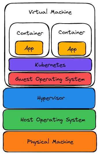
- Kubeflow makes use of Kubernetes, a container orchestrator, which means that the distributed training will be run as a group of containers running in parallel and synchronizing with one another.
Creating a yaml file defining training parameters
- Training parameters include image name, the command to run, volume and network file system access, number of workers, number of GPUs in each worker, etc.
- Check the GAN PyTorchJob file used for more information.
The distributed training strategy used for training the GAN for producing hadronic showers in the calorimeter detectors is DistributedDataParallel from PyTorch, which provides data parallelism by synchronizing gradients across each model replica.
Training Time
Let’s start by training the model on 4, 8, 16, and 32 A100 40GB GPUs and compare the results.
| Number of GPUs | Batch Size | Time per Epoch [s] |
|---|---|---|
| 4 | 64 | 210 |
| 8 | 64 | 160 |
| 16 | 64 | 120 |
| 32 | 64 | 78 |
Ideally, when doubling the number of GPUs, we would like to have double the performance. In reality the extra overhead smooths out the performance gain:
| T(4 GPUs) / T(8 GPUs) | T(8 GPUs) / T(16 GPUs) | T(16 GPUs) / T(32 GPUs) |
|---|---|---|
| 1.31 | 1.33 | 1.53 |
Conclusions:
- As expected, as we increase the number of GPUs the time per epoch decreases.
- As we double the number of GPUs, the 30% improvement achieved is lower than expected. This can be caused by multiple things, but one viable option to consider is using a different framework for distributed training. Examples include DeepSpeed or FSDP.
Bringing MIG into the mixture
Next, we can try and perform the same training on MIG-enabled GPUs. In the measurements that follow:
mig-2g.10gb- every GPU is partitioned into 3 instances of 2 compute units and 10 GB virtual memory each (3*2g.10gb).mig-3g.20gb- every GPU is partitioned into 2 instances of 3 compute units and 20 GB virtual memory each (2*3g.20gb).
For more information about MIG profiles check the previous blog post and the upstream NVIDIA documentation. Now we can redo the benchmarking, keeping in mind that:
- The mig-2g.10gb configuration has 3 workers per GPU, and mig-3g.20gb has 2 workers.
- On more powerful instances we can opt for bigger batch sizes to get the best performance.
- There should be no network overhead for MIG devices on the same GPUs.
2g.10gb MIG workers
| Number of A100 GPUs | Number of 2g.10gb MIG instances | Batch Size | Time per Epoch [s] |
|---|---|---|---|
| 4 | 12 | 32 | 505 |
| 8 | 24 | 32 | 286 |
| 16 | 48 | 32 | 250 |
| 32 | 96 | 32 | OOM |
The performance comparison when doubling the number of GPUs:
| T(12 MIG instances) / T(24 MIG instances) | T(24 MIG instances) / T(48 MIG instances) | T(48 MIG instances) / T(96 MIG instances) |
|---|---|---|
| 1.76 | 1.144 | OOM |
Conclusions:
- Huge improvements when scaling from 4 to 8 GPUs, the epoch time decreased from 505 to 286 seconds, about 76%.
- Doubling the number the GPUs again (from 8 to 16) improved the time by only ~14%.
- When fragmenting the training too much, we can encounter OOM errors.
- As we use DistributedDataParallel from PyTorch for data parallelism, the OOM is most likely caused by the extra memory needed to do gradient aggregation.
- It can also be caused by inefficiencies when performing the gradient aggregation, but nccl (the backend used) should be efficient enough. This is something to be investigated later.
3g.20gb MIG workers
| Number of full A100 GPUs | Number of 3g.20gb MIG instances | Batch Size | Time per Epoch [s] |
|---|---|---|---|
| 4 | 8 | 64 | 317 |
| 8 | 16 | 64 | 206 |
| 16 | 32 | 64 | 139 |
| 32 | 64 | 64 | 114 |
The performance comparison when doubling the number of GPUs:
| T(8 MIG instances) / T(16 MIG instances) | T(16 MIG instances) / T(32 MIG instances) | T(32 MIG instances) / T(64 MIG instances) |
|---|---|---|
| 1.53 | 1.48 | 1.21 |
Conclusions:
- When increasing the number of GPUs from 4 to 8, initially the scaling is less aggressive than it was for 2g.10gb instances (53% vs 76%), but it is more stable and allows to further increase the number of GPUs.
mig-3g.20gb vs mig-disabled:
There are some initial assumptions we have, that should lead to the mig-disabled setup being more efficient than mig-3g.20gb. Consult the previous blogpost for more context:
- Double the number of Graphical Instances:
- In the mig-3g.20gb setup, every GPU is partitioned into 2, as a result, we have double the number of GPU instances.
- This results in more overhead.
- The number of SMs:
- For NVIDIA A100 40GB GPU, 1 SM means 64 CUDA Cores and 4 Tensor Cores
- A full A100 GPU has 108 SMs.
- 2 * 3g.20gb mig instances have in total 84 SMs (3g.20gb=42 SMs, consult the previous blog post for more information).
- mig-disabled setup has 22.22% more CUDA cores and Tensor Cores than mig-3g.20gb setup
- Memory:
- The full A100 GPU has 40GB of virtual memory
- 2 * 3g.20gb mig instances have 2 * 20 GB = 40 GB
- no loss of memory
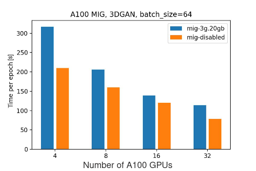
Based on the experimental data, as expected, performing the training on full A100 GPUs shows better results than on mig-enabled ones. This can caused by multiple factors:
- Loss of SMs when enabling MIG
- Communication overhead
- Gradient synchronization
- Network congestion, etc.
At the same time, the trend seems to point out that as we increase the number of GPUs, the difference between mig-disabled vs mig-enabled setup alleviates.
Conclusions
- Although partitioning GPUs can be beneficial for providing bigger GPU offering and better utilization, it is still worth it to have dedicated GPUs for running demanding production jobs.
- Given a setup where GPUs are available but mig-partitioned, distributed training is a viable option:
- It comes with a penalty for the extra communication/bigger number of GPUs to provide same amount of resources.
- Adding small GPU instances can initially speed up the execution, but the improvement will decrease as more overhead is added, and in some cases the GPU will go OOM.
During these tests, we discovered that the training time per epoch varied significantly for the same input parameters (number of workers, batch size, MIG configuration). It led to the topology analysis that follows in the next section.
Topology
Getting variable execution times for fixed inputs lead to some additional investigations. The question is: “Does the topology affect the performance in a visible way?”.
In the following analysis, we have 8 nodes, each having 4 A100 GPUs. Given that we need 16 GPUs for model training, would it be better and more consistent if the workers utilized all 4 GPUs on 4 machines, or if the workers were distributed across more nodes?
To represent topologies, we will use a sequence of numbers, showing how many GPUs were in-use on different nodes.
For example, the topologies below can be represented as 3 2 1 1 1 and 0 0 2 1 1 1 3:
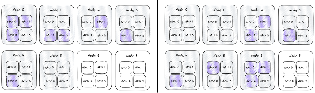
Conceptually all the nodes are the same, and the network behaves uniformly between them, so it shouldn’t matter on which node we schedule the training. As a result the topologies above (0 0 2 1 1 1 3 and 3 2 1 1 1) are actually the same, and can be generically represented as 1 1 1 2 3.
Setup
It seems that when deploying Pytorchjobs, the scheduling is only based on availability of the GPUs. Since there isn’t an automatic way to enforce topology at the node level, the topology was captured using the following procedure:
- Identify schedulable nodes. Begin with four available nodes, then increase to five, six, seven, and eight. Workloads will be assigned to available GPUs by the Kubernetes scheduler. Repeat steps 2 through 5 for each available set of nodes.
- On each GPU, clear memory and delete processes.
- Run a process on each node to monitor GPU utilization (which cards are being used)
- Execute a PyTorchjob with 16 workers.
- Store info about every card utilized from each node and the time of the training job across multiple epochs.
The use case is the same: GAN for producing hadronic showers in the calorimeter detectors, with the batch size of 64. Full A100 GPUs were used for this part, with MIG disabled. The source code for the analysis can be found in this repository.
Analyzing the results
The benchmarking results can be found in the a100_topology_experiment.txt file, but it is pretty hard to make conclusions without visualizing the result.
Each job has three epochs, which are shown in blue, orange, and green. Unfortunately, the number of experiments per topology is not consistent, and can vary from 1 to 20 samples, and at the time of writing the setup cannot be replicated. As a result, take the following observations with a grain of salt.
We try to pinpoint the topologies where the performance is high, but the variance is small. For every topology we have the average excution time, but also how much the value varied across jobs.
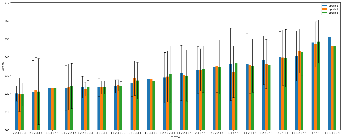
Conclusions
- Even if the topology is fixed, the epoch times vary a lot. For topology
4 4 4 4, the epoch time range from 120 to 160 seconds, even though the whole setup is the same. - The epoch times at the job level do not vary significantly. The main distinction is seen between jobs.
- The best topology is not necessarily the one that produces the best results for a single job, but rather the one that produces the most uniform distribution of results.
- There are some topologies that out-perform others in terms of execution time and stability. By comparing the results it seems that they are skewed towards taking advantage of in-node communication, while leaving resources for bursty behaviour.
- The best results seem to be for
1 2 2 2 3 3 3,3 3 3 3 4, and1 1 2 3 3 3 3topologies. The common point for them is that they take advantage of 3/4 GPUs on the nodes, as a result having fast in-node communication but also making sure there is no GPU congestion.
- The best results seem to be for
This analysis is done at a fairly high level. To gain a better understanding of the performance, we should investigate the NUMA settings. Additionally, different synchronization strategies, such as parameter server, could be used to achieve more consistent performance.