Efficient Access to Shared GPU Resources: Part 5
This is part 5 of a series of blog posts about GPU concurrency mechanisms. In part 1 we focused on the pros and cons of different solutions available on Kubernetes, in part 2 we dove into the setup and configuration details, in part 3 we analyzed the benchmarking use cases, and in part 4 we benchmarked the time slicing mechanism.
In this part 5 we will focus on benchmarking MIG (Multi-Instance GPU) performance of NVIDIA cards.
This series focuses on NVIDIA cards, although similar mechanisms might be offered by other vendors.
Setup
The benchmark setup will be the same for every use case:
- Full GPU (MIG disabled) vs MIG enabled (7g.40gb partition)
- MIG enabled, different partitions:
- 7g.40gb
- 3g.20gb
- 2g.10gb
- 1g.5gb
Keep in mind that the nvidia-smi command will not return the GPU utilization if MIG is enabled. This is the expected behaviour, as NVML (NVIDIA management library) does not support attribution of utilization metrics to MIG devices. For monitoring MIG capable GPUs it is recommended to rely on NVIDIA DCGM instead.
Find more about the drivers installation, MIG configuration, and environment setup.
Theoretical MIG performance penalty
When sharing a GPU between multiple processes using time slicing, there is a performance loss caused by the context switching. As a result, when enabling time slicing but scheduling a single process on the GPU, the penalty can be neglected.
On the other hand, with MIG, the assumptions are very different. By just enabling MIG, a part of the Streaming Multiprocessors are lost. But there is no additional penalty introduced when further partitioning the GPU.
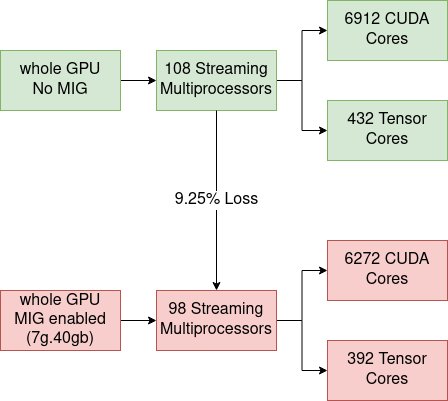
For instance, as can be seen in the image below, a whole A100 40GB NVIDIA GPU (the GPU used for the benchmarking that follows) has 108 Streaming Multiprocessors (SMs). When enabling MIG, 10 SMs are lost, which is the equivalent of 9.25% of the total number of compute cores.
As a result, when enabling MIG, it is expected to see a performance penalty of ~9.25%. As partitions are considered isolated, we shouldn’t have additional overhead when sharing the GPU between many users. We expect the scaling between partitions to be linear, meaning a 2g.10gb partition should perform 2 times better than a 1g.5gb because it has double the resources.
FLOPS Counting
Floating Point Operations Per Second (FLOPS) is the metric used to show how powerful a GPU is when working with different data formats. To count FLOPS we rely on dcgmproftester, a CUDA-based test load generator from NVIDIA. For more information, consult the previous blog post.
Full GPU (MIG disabled) vs MIG enabled (7g.40gb partition)
| Formats | Full GPU (MIG disabled) [TFLOPS] | MIG enabled (7g.40gb) [TFLOPS] | Loss [%] |
|---|---|---|---|
| fp16, Cuda Cores | 32.785 | 30.583 | 6.71 |
| fp32, Cuda Cores | 16.773 | 15.312 | 8.71 |
| fp64, Cuda Cores | 8.128 | 7.386 | 9.12 |
| fp16, Tensor Cores | 164.373 | 151.701 | 7.70 |
FLOPS counting per MIG partition
| Formats | 7g.40gb [TFLOPS] | 3g.20gb [TFLOPS] | 2g.10gb [TFLOPS] | 1g.5gb [TFLOPS] | |
|---|---|---|---|---|---|
| fp16, Cuda Cores | 30.583 | 13.714 | 9.135 | 4.348 | |
| fp32, Cuda Cores | 15.312 | 6.682 | 4.418 | 2.132 | |
| fp64, Cuda Cores | 7.386 | 3.332 | 2.206 | 1.056 | |
| fp16, Tensor Cores | 151.701 | 94.197 | 65.968 | 30.108 |
FLOPS scaling between MIG partitions
| Formats | 7g.40gb / 3g.20gb | 3g.20gb / 2g.10gb | 2g.10gb / 1g.5gb |
|---|---|---|---|
| fp16, Cuda Cores | 2.23 | 1.50 | 2.10 |
| fp32, Cuda Cores | 2.29 | 1.51 | 2.07 |
| fp64, Cuda Cores | 2.21 | 1.51 | 2.08 |
| fp16, Tensor Cores | 1.61 | 1.42 | 2.19 |
| Ideal Scale | 7/3=2.33 | 3/2=1.5 | 2/1=2 |
Memory bandwidth scaling between MIG partitions
| Partition | Memory bandwidth | Multiplying factor |
|---|---|---|
| 7g.40gb | 1555.2 GB | 8 |
| 3g.20gb | 777.6 GB | 4 |
| 2g.10gb | 388.8 GB | 2 |
| 1g.5gb | 194.4 GB | 1 |
Conclusions
- Enabling MIG:
- For fp32 and fp64, Cuda Cores, the drop in performance is close to the theoretical one.
- For fp16 on Cuda Cores and Tensor Cores, the loss is much smaller than the expected value. Might need further investigation.
- There is no loss of memory bandwidth.
- The scaling between partitions:
- On CUDA Cores (fp16, fp32, fp64) the scaling is converging to the theoretical value.
- On Tensor Cores the scaling diverges a lot from the expected one (especially when comparing 7g.40gb and 3g.20gb). Might need further investigation.
- The scaling of the memory bandwidth is based on powers of 2 (1, 2, 4, and 8 accordingly).
Compute-Intensive Particle Simulation
An important part of CERN computing is dedicated to simulation. These are compute-intensive operations that can significantly benefit from GPU usage. For this benchmarking, we rely on the lhc simpletrack simulation. For more information, consult the previous blog post.
Full GPU (MIG disabled) vs MIG enabled (7g.40gb partition)
| Number of particles | Full GPU (MIG disabled) [seconds] | MIG enabled (7g.40gb) [seconds] | Loss [%] |
|---|---|---|---|
| 5 000 000 | 26.365 | 28.732 | 8.97 |
| 10 000 000 | 51.135 | 55.930 | 9.37 |
| 15 000 000 | 76.374 | 83.184 | 8.91 |
Running simulation on different MIG partitions
| Number of particles | 7g.40gb [seconds] | 3g.20gb [seconds] | 2g.10gb [seconds] | 1g.5gb [seconds] | |
|---|---|---|---|---|---|
| 5 000 000 | 28.732 | 62.268 | 92.394 | 182.32 | |
| 10 000 000 | 55.930 | 122.864 | 183.01 | 362.10 | |
| 15 000 000 | 83.184 | 183.688 | 273.700 | 542.300 |
Scaling between MIG partitions
| Number of particles | 3g.20gb / 7g.40gb | 2g.10gb / 3g.20gb | 1g.5gb / 2g.10gb |
|---|---|---|---|
| 5 000 000 | 2.16 | 1.48 | 1.97 |
| 10 000 000 | 2.19 | 1.48 | 1.97 |
| 15 000 000 | 2.20 | 1.49 | 1.98 |
| Ideal Scale | 7/3=2.33 | 3/2=1.5 | 2/1=2 |
Conclusions
- The performance loss when enabling MIG is very close to the theoretical 9.25%.
- The scaling between partitions converges to the ideal values.
- The results are very close to the theoretical assumptions because the benchmarked script is very compute-intensive, without many memory accesses, being CPU bound, etc.
Machine Learning Training
For benchmarking, we will use a pre-trained model and fine-tune it with PyTorch. To maximize GPU utilization, make sure the script is not CPU-bound, by increasing the number of data loader workers and batch size. More details can be found in the previous blog post.
Full GPU (MIG disabled) vs MIG enabled (7g.40gb partition)
- dataloader_num_workers=8
- per_device_train_batch_size=48
- per_device_eval_batch_size=48
| Dataset size | Full GPU (MIG disabled) [seconds] | MIG enabled (7g.40gb) [seconds] | Loss [%] |
|---|---|---|---|
| 2 000 | 63.30 | 65.77 | 3.90 |
| 5 000 | 152.91 | 157.86 | 3.23 |
| 10 000 | 303.95 | 313.22 | 3.04 |
| 15 000 | 602.70 | 622.24 | 3.24 |
7g.40gb vs 3g.20gb
- per_device_train_batch_size=24
- per_device_eval_batch_size=24
- dataloader_num_workers=4
| Dataset size | 7g.40gb [seconds] | 3g.20gb [seconds] | 3g.20gb / 7g.40gb (Expected 7/3=2.33) |
|---|---|---|---|
| 2 000 | 67.1968 | 119.4738 | 1.77 |
| 5 000 | 334.2252 | 609.2308 | 1.82 |
| 10 000 | 334.2252 | 609.2308 | 1.82 |
When comparing a 7g.40gb instance vs a 3g.20gb one, the amount of cores becomes 2.33 (7/3) times smaller. This is the scale we are expecting to see experimentally as well, but the results are converging to 1.8 rather than 2.3. For machine learning training, the results are influenced a lot by the available memory, bandwidth, how the data is stored, how efficient the data loader is, etc.
To simplify the benchmarking, we will use the 4g.20gb partition instead of the 3g.20gb. This way all the resources (bandwidth, cuda cores, tensor cores, memory) are double when compared to 2g.10gb, and the ideal scaling factor is 2.
4g.20gb vs 2g.10gb:
- per_device_train_batch_size=12
- per_device_eval_batch_size=12
- dataloader_num_workers=4
| Dataset size | 4g.20gb [seconds] | 2g.10gb [seconds] | 2g.10gb / 4g.20gb (Expected 4/2=2) |
|---|---|---|---|
| 2 000 | 119.2099 | 223.188 | 1.87 |
| 5 000 | 294.6218 | 556.4449 | 1.88 |
| 10 000 | 589.0617 | 1112.927 | 1.88 |
2g.10gb vs 1g.5gb:
- per_device_train_batch_size=4
- per_device_eval_batch_size=4
- dataloader_num_workers=2
| Dataset size | 2g.10gb [seconds] | 1g.5gb [seconds] | 1g.5gb / 2g.10gb (Expected 2/1=2) |
|---|---|---|---|
| 2 000 | 271.6612 | 525.9507 | 1.93 |
| 5 000 | 676.3226 | 1316.2178 | 1.94 |
| 10 000 | 1356.9108 | 2625.1624 | 1.93 |
Conclusions
- The performance loss when enabling MIG is much smaller than the theoretical 9.25%. This can be caused by many reasons:
- complex operations to be performed
- being IO bound
- executing at a different clock frequency
- variable tensor core utilization, etc.
- The training time depends heavily on the number of CUDA Cores, Tensor Cores, but also the memory bandwidth, the data loader, the batch size, etc. Consult the previous blog for some ideas on how to profile and detect performance bottlenecks of models.
- The scaling between partitions is linear and is converging to the expected value. Especially on smaller partitions.
Takeaways
- When using MIG technology, the GPU partitions are isolated and can run securely without influencing each other.
- A part of the available streaming multiprocessors are lost when enabling MIG:
- In the case of an A100 40GB NVIDIA GPU, 10/108 SMs, which means losing 9.25% of the available Cuda and Tensor cores.
- Never enable MIG without actually partitioning the GPU (the 7g.40gb partition). It means losing performance without gaining GPU sharing.
- When enabling MIG:
- The performance loss for compute-intensive applications can reach ~9.25%.
- For machine learning training the loss alleviates as a result of memory accessing, being IO bound, being CPU bound, etc, and experimentally it will be much smaller than expected.
- The scaling between partitions is linear. Doubling the resources halves the execution time.
- For GPU monitoring rely on NVIDIA Data Center GPU Manager (DCGM). It is a suite of tools that includes active health monitoring, diagnostics, power and clock management, etc.
- A current limitation (with CUDA 11/R450 and CUDA 12/R525) that might be relaxed in the future is that regardless of how many MIG devices are created (or made available to a container), a single CUDA process can only enumerate a single MIG device. The implications are:
- We cannot use 2 MIG instances in a single process.
- If at least one device is in MIG mode, CUDA will not see the non-MIG GPUs.
Next episode
In the next blog post, we will use NVIDIA A100 GPUs and MIG to train in distributed mode a high energy physics (HEP) neural network on-prem Kubeflow. Stay tuned!