This is the multi-page printable view of this section. Click here to print.
News About Kubernetes
- Fault Tolerance Solutions for Multi-Cluster Kubernetes: Part 1
- Rootless container builds on Kubernetes
- autofs in containers
- GitLab Runners and Kubernetes: A Powerful Duo for CI/CD
- Nurturing Sustainability: Raising Power Consumption Awareness
- Efficient Access to Shared GPU Resources: Part 6
- Webinar: Fully Automated Deployments with ArgoCD
- Efficient Access to Shared GPU Resources: Part 5
- Webinar: Container Storage Improved: What's New in CVMFS and EOS Integrations
- Efficient Access to Shared GPU Resources: Part 4
- Propagating OAuth2 tokens made easier
- Efficient Access to Shared GPU Resources: Part 3
- Efficient Access to Shared GPU Resources: Part 2
- Efficient Access to Shared GPU Resources: Part 1
- Announcing CVMFS CSI v2
- A Summer of Testing and Chaos
- Summary of the GitOps Workshop
- GitOps Workshop
- Kubernetes Deprecations and Removals v1.20/21/22
Fault Tolerance Solutions for Multi-Cluster Kubernetes: Part 1
Supervisor: Jack Munday
My summer at CERN OpenLab
This summer I had the opportunity to work as a summer student at CERN OpenLab, where I was part of the IT-CD team. My project focused on implementing fault tolerance solutions for multi-cluster Kubernetes deployments, specifically using Cilium Cluster Mesh and various database technologies. The goal was to ensure high availability and redundancy for user traffic and databases across multiple clusters.
I had a great summer at CERN, I learnt a lot both professionally and personally, and I had the chance to meet many interesting people. Without further a do, let’s go into it!

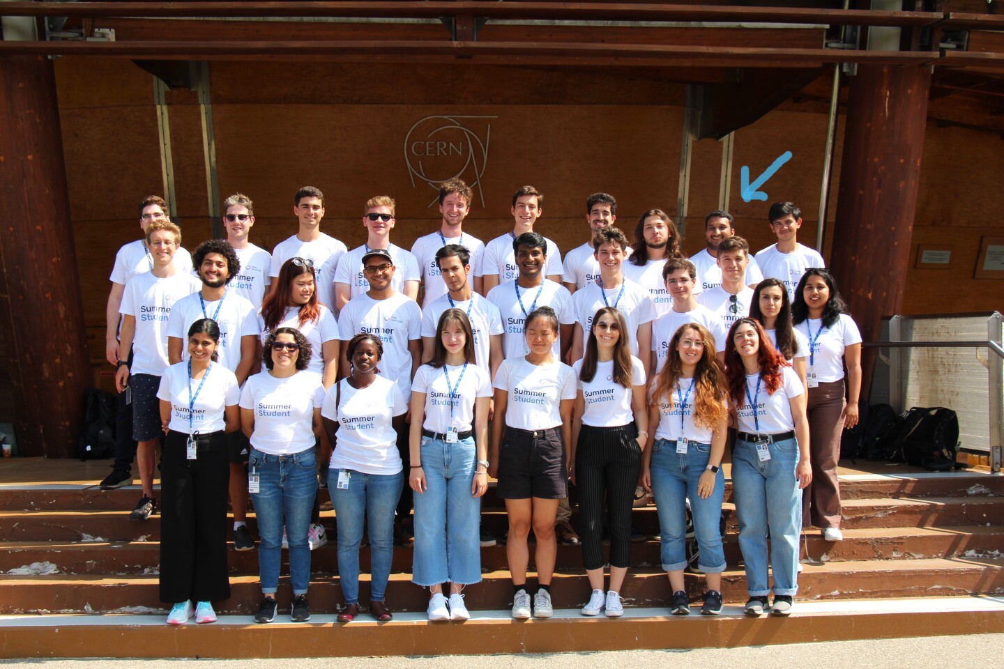
OpenLab Summer Students class of 2025.
Introduction
High Availability is the design of systems and services to ensure they remain operation and accessible with minimal downtime, even in the face of server failures. It is a broader field of Business Continuity, which is a set of strategies to keep business operations during and after disruptions. The four levels of Business Continuity are described in the diagram below. The levels go from Cold with hours or even days of downtime, to Active-Active with practically no downtime.

Levels of Business Continuity. Inspired by CERN’s BC/DR Team.
In these two articles, we will focus on Active-Active and Active-Passive levels. Active-Active is a configuration where multiple clusters are running the same application simultaneously, sharing the load and providing redundancy. Active-Passive is a configuration where one cluster is active and serving requests, while another cluster is on standby, ready to take over in case of failure. In the context of this article, Active-Passive only provides redundancy for databases, which are continuously replicated across clusters. In the table above, the Active-Passive covers all the levels before Active-Active. The second article is about Active-Passive and is released on this same blog.
Active-Active Setup for Applications
Cilium is a Kubernetes CNI (Container Network Interface) plugin that provides advanced networking and security features for Kubernetes clusters. It is designed to enhance the performance, scalability, and security of containerized applications. Cilium uses eBPF (extended Berkeley Packet Filter) technology to implement networking and security policies at the kernel level, allowing for efficient and flexible network management.
Cilium Cluster Mesh is a feature that allows multiple Kubernetes clusters to be connected and managed as a single logical network. This enables seamless communication between pods across different clusters. Cluster Mesh is particularly useful for multi-cluster deployments, where applications need to span multiple clusters for high availability. This feature differs from service mesh, which is a layer that provides communication between services within a cluster, whereas Cluster Mesh focuses on communication between clusters.
The benefit of Cilium Cluster Mesh is that it allows for seamless communication between pods across different clusters, enabling load balancing and failover capabilities. It allows user traffic to be distributed across multiple clusters, ensuring that if one cluster fails, the other clusters can continue to serve requests. Furthermore, with Cilium Cluster Mesh it is seamless to label services as global, which allows them to be discovered and accessed from any cluster in the mesh. This way it is also easy to group pods together, as the pods with the same names in different groups perform the load balancing just between each other.
This chapter will cover the setup of Cilium Cluster Mesh for Active-Active user traffic. The setup involves configuring multiple pods in different clusters, and then load balancing the traffic across these pods. The goal is to ensure that user requests are distributed evenly across the clusters, providing redundancy and high availability even if one of the clusters fail. The diagram below illustrates the architecture used for this setup, with the API- and ML-services running in different clusters, and the user traffic being load balanced across them pairwise.

Cilium Cluster Mesh architecture.
Cilium Cluster Mesh Basic Installation
Installing Cilium and Cilium Cluster Mesh is straightforward with the Cilium CLI, and you can follow this guide by Cilium to get it installed.
However, users may encounter issues with the Cilium Cluster Mesh installation via Cilium CLI, especially if they have a larger umbrella Helm chart for all their installations. Furthermore, when running the cilium clustermesh connect command on the CLI installation, the Cilium installation exceeded Helm release size limit of 1 MB. To overcome this, one can install Cilium Cluster Mesh manually with Helm. Let’s assume that one has two clusters named cilium-001and cilium-002, both with certmanager installed. On a high level, it can be done as follows:
- Create the Kubernetes clusters and install Cilium in them via Helm.
# Run this against both of the Kubernetes clusters.
helm repo add cilium https://helm.cilium.io/
helm install -n kube-system cilium cilium/cilium --create-namespace --version 1.18.0
- We ran multiple helm upgrades to register and mesh our clusters together. First installing cilium with
clustermesh.useAPIServer=trueand then enablingclustermeshin a subsequent upgrade with the relevant configuration for all clusters. Below is presented the final configuration for brevity for cilium-002, the configuration for cilium-001 is similar with a different CIDR range and the certificates for cilium-002 instead.
---
# cilium-002.yaml
cilium:
  cluster:
    name: <CILIUM-002-MASTER-NODE-NAME>  # Master node name from `kubectl get no`
    id: 002 # Cluster ID, can be any number, but should be unique across clusters.
  ipam:
    operator:
      clusterPoolIPv6MaskSize: 120
      clusterPoolIPv4MaskSize: 24
      clusterPoolIPv6PodCIDRList:
        - 2001:4860::0/108
      clusterPoolIPv4PodCIDRList: # Ensure each cluster in your mesh uses a different CIDR range.
        - 10.102.0.0/16
  bpf:     # Mandatory to fix issue mentioned in https://github.com/cilium/cilium/issues/20942
    masquerade: true
  clustermesh:
   apiserver:
    tls:
      server:
        extraDnsNames:
          - "*.cern.ch" # If you are relying on cilium to generate your certificates.
    useAPIServer: true
    config:
      enabled: true
      domain: cern.ch
      clusters:
        - name: <CILIUM-001-MASTER-NODE-NAME> # Second cluster master node name from kubectl get no.
          port: 32379
          ips:
            - <CILIUM-001-MASTER-NODE-IP> # Second cluster internal IP address from kubectl get no -owide.
          tls: # Certificates can be retrieved with `kubectl get secret -n kube-system clustermesh-apiserver-remote-cert -o jsonpath='{.data}'`
            key: <APISERVER-KEY>
            cert: <APISERVER-CERT>
            caCert: <APISERVER-CA-CERT>
Load Balancer Setup
To enable external access to the cluster with this integration, an ingress must be deployed, which in turn automatically provisions a load balancer for the cluster. Ingress-nginx ingress controller is used for this purpose, as with Cilium ingress controller I encountered problems with the cluster networking (see more in the Troubleshooting section). Install the ingress-nginx controller with the following Helm configuration:
# cilium-002-ingress-controller.yaml
ingress-nginx:
  controller:
    nodeSelector:
      role: ingress
    service:
      enabled: true
      nodePorts:
        http: ""
        https: ""
      type: LoadBalancer
  enabled: true
Since the Helm configuration deployed the load balancer into a node with label ingress, we should label one as such, preferably before the ingress-nginx installation:
kubectl label node <NODE-OF-CHOICE> role=ingress
Next up, we should deploy the ingress and thus the load balancer by applying this custom resource definition (CRD):
# ingress-manifest.yaml
apiVersion: networking.k8s.io/v1
kind: Ingress
metadata:
  name: sample-http-ingress
  annotations:
    # This annotation added to get the setup to work
    # Read more at https://github.com/cilium/cilium/issues/25818#issuecomment-1572037533
    # and at https://github.com/kubernetes/ingress-nginx/blob/main/docs/user-guide/nginx-configuration/annotations.md#service-upstream
    nginx.ingress.kubernetes.io/service-upstream: "true"
spec:
  ingressClassName: nginx
  rules:
  - host:
    http:
      paths:
      - path: /
        pathType: Prefix
        backend:
          service:
            name: api-service # Name of a global service backend. If you would deploy another service, you would need to change this name to ML-service or something else.
            port:
              number: 8080
Deploy this CRD with kubectl apply -f ingress-manifest.yaml. The load balancer will be provisioned automatically, and the ingress controller will start routing traffic to the specified backend service later. Apply this in both clusters. Then, configure DNS load balancing by assigning the same DNS name to the external addresses of both load balancers. This way, when clients resolve the DNS name, the DNS service distributes requests across the available load balancers. This step depends on the DNS service you are using.
Global Services
The automatic load-balancing between clusters can be achieved by defining Kubernetes ClusterIP services with identical names and namespaces and by adding the annotation service.cilium.io/global: "true" to declare them global. Cilium will take care of the rest. Furthermore, since this guide is utilizing an external ingress controller, an additional annotation is needed for the global services, namely service.cilium.io/global-sync-endpoint-slices: "true". Apply the following CRD in both of the clusters to create the global service ClusterIP, and mock pods within them:
# global-api-service-manifest.yaml
apiVersion: v1
kind: Service
metadata:
  # The name and namespace need to be the same across services in different clusters. This name is important as it defines the load balancing groups for Cilium.
  name: api-service
  annotations:
    # Declare the global service.
    # Read more here: https://docs.cilium.io/en/stable/network/clustermesh/services/
    service.cilium.io/global: "true"
    # Allow the service discovery with third-party ingress controllers.
    service.cilium.io/global-sync-endpoint-slices: "true"
spec:
  type: ClusterIP
  ports:
  - name: http
    protocol: TCP
    port: 8080
    targetPort: 80
  selector:
    app: api-service
---
apiVersion: apps/v1
kind: Deployment
metadata:
  name: api-service
spec:
  replicas: 1
  selector:
    matchLabels:
      app: api-service
  template:
    metadata:
      labels:
        app: api-service
    spec:
      containers:
      - name: nginx
        image: nginx
        ports:
        - containerPort: 80
        volumeMounts:
        - name: html
          mountPath: /usr/share/nginx/html/index.html
          subPath: index.html
      volumes:
      - name: html
        configMap:
          name: custom-index-html
---
apiVersion: v1
kind: ConfigMap
metadata:
  name: custom-index-html
data:
  # Hello from Cluster 001 or Cluster 002, depending on the cluster.
  index.html: |
    Hello from Cluster 00x
Deploy with kubectl apply -f global-api-service-manifest.yaml, after which one can check that the global service is working by checking that we can get responses from both of the clusters:
# Run a pod which can access the cluster services.
kubectl run curlpod --rm -it --image=busybox -- sh
# This should return "Hello from Cluster 001" or "Hello from Cluster 002" depending on which cluster the request was routed to.
wget -qO- http://api-service:8080
Testing Cluster Mesh Connectivity
Now everything should be working. You can test the solution in many ways, below listed a couple methods:
- By using Cilium CLI (needs Cilium CLI installed):
# To check that normal Cilium features are working.
cilium status

# Expected output
    /¯¯\
/¯¯\__/¯¯\    Cilium:             OK
\__/¯¯\__/    Operator:           OK
/¯¯\__/¯¯\    Envoy DaemonSet:    OK
\__/¯¯\__/    Hubble Relay:       OK
    \__/       ClusterMesh:        OK

DaemonSet              cilium                   Desired: 2, Ready: 2/2, Available: 2/2
DaemonSet              cilium-envoy             Desired: 2, Ready: 2/2, Available: 2/2
Deployment             cilium-operator          Desired: 2, Ready: 2/2, Available: 2/2
Deployment             clustermesh-apiserver    Desired: 1, Ready: 1/1, Available: 1/1
Deployment             hubble-relay             Desired: 1, Ready: 1/1, Available: 1/1
Deployment             hubble-ui                Desired: 1, Ready: 1/1, Available: 1/1
Containers:            cilium                   Running: 2
                       cilium-envoy             Running: 2
                       cilium-operator          Running: 2
                       clustermesh-apiserver    Running: 1
                       hubble-relay             Running: 1
                       hubble-ui                Running: 1
Cluster Pods:          27/27 managed by Cilium
Helm chart version:    1.17.5
Image versions         cilium                   quay.io/cilium/cilium:v1.17.5 2
                       cilium-envoy             quay.io/cilium/cilium-envoy:v1.32.7 2
                       cilium-operator          quay.io/cilium/operator-generic:v1.17.5 2
                       clustermesh-apiserver    quay.io/cilium/clustermesh-apiserver:v1.17.5 3
                       hubble-relay             quay.io/cilium/hubble-relay:v1.17.5 1
                       hubble-ui                quay.io/cilium/hubble-ui-backend:v0.13.2 1
                       hubble-ui                quay.io/cilium/hubble-ui:v0.13.2@sha256 1
# To check if Cluster Mesh installation is working. You can run this both on cilium-001 and cilium-002 clusters, and the output should be similar in both. Example ran on cilium-001. cilium clustermesh status # Expected output ⚠️ Service type NodePort detected! Service may fail when nodes are removed from the cluster! ✅ Service "clustermesh-apiserver" of type "NodePort" found ✅ Cluster access information is available: - <CILIUM-001-MASTER-IP>:32379 ✅ Deployment clustermesh-apiserver is ready ℹ️ KVStoreMesh is enabled ✅ All 2 nodes are connected to all clusters [min:1 / avg:1.0 / max:1] ✅ All 1 KVStoreMesh replicas are connected to all clusters [min:1 / avg:1.0 / max:1] 🔌 Cluster Connections: - <CILIUM-002-MASTER-NODE-NAME>: 2/2 configured, 2/2 connected - KVStoreMesh: 1/1 configured, 1/1 connected 🔀 Global services: [ min:1 / avg:1.0 / max:1 ]# To test the Cluster Mesh connection. # Assumes that you have set up kubectl contexts for the clusters. # To test the Cluster Mesh pod connectivity. cilium connectivity test --context <CLUSTER-1-CTX> --destination-context <CLUSTER-2-CTX> - Verifying that you can see pods with identities in both clusters:
kubectl exec -it -n kube-system $(kubectl get pods -n kube-system -l k8s-app=cilium -o jsonpath='{.items[0].metadata.name}') -c cilium-agent -- cilium-dbg node list | awk '{print $1}'

Name
cilium-001-master-0/cilium-001-master-0
cilium-001-master-0/cilium-001-node-0
cilium-002-master-0/cilium-002-master-0
cilium-002-master-0/cilium-002-node-0
- By curling ingress-nginx load balancer with load balancer IP or DNS:
# Run either one of these two to get the IP.
kubectl get ingress sample-http-ingress -o yaml
openstack loadbalancer list
# Use either IP or DNS to curl the system.
curl <DNS-NAME> -v
curl http://<LB-IP>:8080 -v

# Expected output:
# Hello from Cluster 001
# Hello from Cluster 002
The Cluster Mesh connectivity refers to the ability of Cilium to route requests to pods in both clusters. It works non-deterministically, and if a pod in the local or remote cluster breaks, the requests are routed to the working cluster.
The failover was tested by downscaling the replicas of the API-service in one cluster, and then checking that the requests were routed to the other cluster. The failover worked as expected, and the requests were routed to the working cluster.
Troubleshooting
bpf.masquerade=truein the Cilium Helm configuration is required as stated here.- Cilium also offers an ingress controller. I experimented with it with the following YAML:
However, I encountered issues with the cluster networking, and it did not work as expected. I was able to query the ingress controller from within the cluster, but when I tried to enable the host network and query the node IP address, I did not get a response. Cilium ingress controller did not require the
bpf: masquerade: false ingressController: enabled: true hostNetwork: enabled: true nodes: matchLabels: role: ingress sharedListenerPort: 8010 service: externalTrafficPolicy: null type: ClusterIPservice.cilium.io/global-sync-endpoint-slices: "true"annotation, as it is already integrated with Cilium Cluster Mesh.
Next Up
In the next article, I will cover the Active-Passive setup for databases, we will cover setting up PostgreSQL, Valkey and OpenSearch with multi-cluster data replication. The goal is to ensure that databases are continuously replicated across clusters, providing redundancy and high availability in case of cluster failures.
References
Rootless container builds on Kubernetes
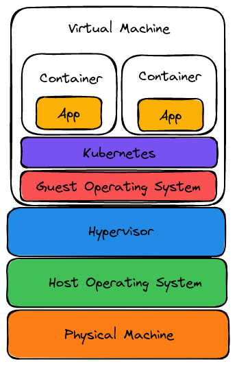
An important task in most teams’ pipelines is building container images. Developers need their builds to be fast, reproducible, reliable, secure and cost-effective. The most isolated setup one can have in a cloud environment is running builds in an isolated server physical or virtual. Spinning new virtual machines (or physical in some cases) is quite easy in cloud environments, but it adds a lot of overhead, provisioning, monitoring, resource usage etc. On the other hand, running builds on a shared host can be insecure in non-trusted environments. Traditionally, dockerd had to be run as root or with root privileges and access to the docker socket was the same as being root. Podman had the same requirements initially as well. In a shared environment (a shared linux host), the most secure option is to run everything as non-root, for additional isolation user namespaces can also be used.
“In Kubernetes v1.33 support for user namespaces is enabled by default!”, this was a big announcement from the cloud-native community earlier this year. Not just because of the feature availability, it has been in beta since v1.30, but because of the maturity of the tooling around it. Improvements had to be made in the Linux Kernel, containerd, cri-o, runc, crun and Kubernetes itself. All this work improved the capabilities of these tools to run workloads rootless.
In this post, we will present 3 options (podman/buildah, buildkit and kaniko) for building container images in Kubernetes pods as non-root with containerd 2.x as runtime. Further improvements can be made using kata-containers, firecracker, gvisor or others but the complexity increases and administrators have to maintain multiple container runtimes.
Podman and Buildah
Podman is a tool to manage OCI containers and pods. Buildah is a tool that facilitates building Open Container Initiative (OCI) container images. Podman vendors buildah’s code for builds, so we can consider it the same. Both CLIs resemble the docker build CLI, and they can be used as drop-in replacements in existing workflows.
To run podman/buildah in a pod we can create an emptyDir volume to use for storage and set a limit to it and also point the run root directory to that volume as well. Then we can runAsUser 1000 (the podman/buildah user in the respective images).
Here is the storage configuration (upstream documentation: storage.conf):
[storage]
driver = "overlay"
runroot = "/storage/run/containers/storage"
graphroot = "/storage/.local/share/containers/storage"
rootless_storage_path = "/storage/.local/share/containers/storage"
[storage.options]
pull_options = {enable_partial_images = "true", use_hard_links = "false", ostree_repos=""}
[storage.options.overlay]
For both buildah and podman we need to configure storage with the overlay
storage driver for good performance. vfs is also an option (driver = "vfs")
but it is much slower especially for big images. Linked are the full manifests
for buildah and podman.
We need the following options:
- place storage.conf in
/etc/containers/storage.confor~/.config/containers/storage.confand mount an emptyDir volume in/storage, we can also configure a size limit... volumeMounts: - name: storage mountPath: /storage - name: storage-conf mountPath: /etc/containers/ volumes: - name: storage emptyDir: sizeLimit: 10Gi - name: storage-conf configMap: name: storage-conf - disable host users to enable user namespaces and run as user
1000... spec: hostUsers: false containers: - name: buildah securityContext: runAsUser: 1000 runAsGroup: 1000 ... - finally build with:
buildah/podman build -t example.com/image:dev .
Buildkit
Buildkit is a project responsible for building artifacts and it’s the project behind the docker build command for quite some time. If you’re using a recent docker you are already using buildkit. docker buildx is a CLI plugin to add extended build capabilities with BuildKit to the docker CLI. Apart from the docker CLI, buildctl and nerdctl can be used against buildkit.
Here is the full example with buildkit based on the upstream example.
To build with buildkit we need to:
- use the buildkit image
docker.io/moby/buildkit:masteror pin to a version egdocker.io/moby/buildkit:v0.23.1 - mount a storage volume (similar to buildah/podman) and specify the storage
directory
BUILDKITD_FLAGS="--root=/storage"... volumeMounts: - name: storage mountPath: /storage volumes: - name: storage emptyDir: sizeLimit: 10Gi - run privileged but with host users disabled
... spec: hostUsers: false containers: - name: buildkit securityContext: # privileged in a user namespace privileged: true ... - for standalone builds we can use buildctl-daemonless.sh a helper script
inside the image
buildctl-daemonless.sh \
  build \
  --frontend dockerfile.v0 \
  --local context=/workspace \
  --local dockerfile=/workspace
We can not use buildkit rootless with user namespaces, rootlesskit needs to be
able to create user mappings. User namespaces can be used with rootful
buildkit, where root is mapped to a high number user, so not really root or
privileged on the host. Here is the rootless upstream
example,
it needs --oci-worker-no-process-sandbox use the host PID namespace and procfs (WARNING: allows build containers to kill (and potentially ptrace) an arbitrary process in the host namespace).
Instead of using buildctl-daemonless.sh or just buildctl, the docker CLI can be used.
docker CLI full example:
cd /workspace
docker buildx create --use --driver remote --name buildkit unix:///path/to/buildkitd.sock
docker buildx build -t  example.com/image:dev .
Kaniko
Kaniko is a tool to build container images from a Dockerfile, inside a container or Kubernetes cluster. Kaniko is stable for quite some time and works without any storage configuration in kubernetes pods. Recently the project was deprecated by Google, but Chainguard is stepping up to maintain it. The debug tags of kaniko’s image contain a shell which is handy for CI pipelines.
To build with kaniko we do not need to mount any volumes for storage. Here is the full example with kaniko.
/kaniko/executor \
  --context /workspace \
  --dockerfile Dockerfile \
  --destination example.com/image:dev \
  --no-push
Performance and resource consumption
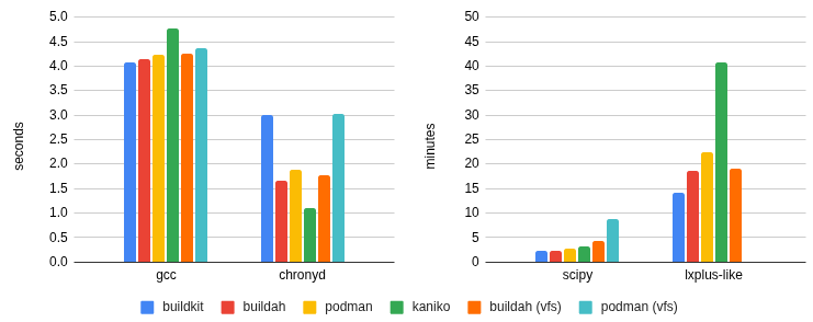
To compare the performance between all tools and try to spot differences, 4 build examples follow.
- gcc based on alpine:latest
- chronyd based on alpine, upstream project.
- jupyter notebook scientific python stack (scipy), upstream project.
- a CERN development environment based on Alma Linux (lxplus), which includes tools like: python, root.cern, HTcondor CLI, kubectl, helm, nvidia cuda toolkit, infiniband and others. Its size is ~35GB/20GB un/compressed, unfortunately it is an internal project.
The builds for gcc and chronyd take less than 5 seconds for all tools. Comparing resource consumption does not add any value. Especially for CIs, the build job may take longer to start or get scheduled.
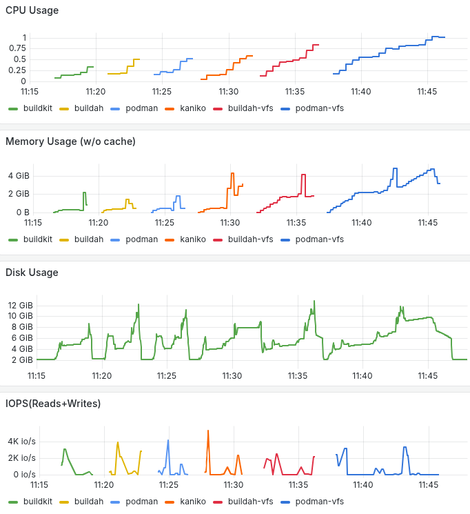
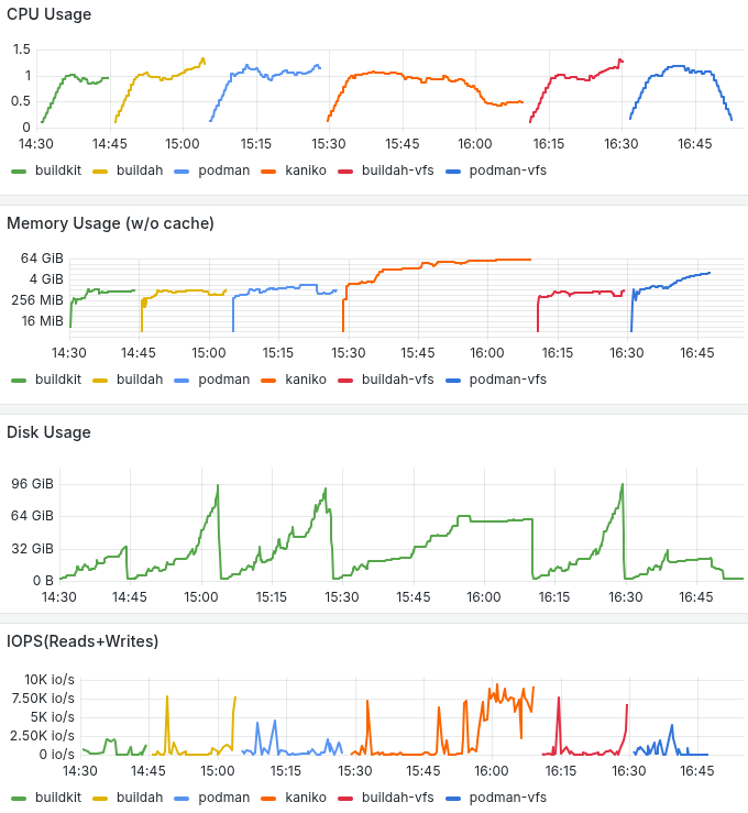
Moving on to build scipy and lxplus which are bigger images with a lot more files we start to see significant differences in build time and resource consumption. Buildkit and buildah/podman configured with overlayfs and overlay respectively, give faster build times, lower memory consumtion and better disk utilization. For the largest image, buildkit’s disk usage efficiency stands out. Below you can go through the build times and resource consumption based on kube-prometheus-stack.
Build time per experiment and per tool:
Pod resource consumption building scipy-notebook.
Pod resource consumption building CERN development environment.
Conclusion
With several improvements being done in past years, building containers as non-root has become much easier. All the mentioned tools provide similar functionality like caching. But which tool to choose?
- For all tools container images are available and good documentation is available.
- For most use cases, the build tool does not matter and the result is the same.
- Buildkit and buildah/podman are fast and do not consume a lot of resources (CPU/RAM). Kaniko has a different approach, for large images it may consume a lot of memory and it can be slower.
- Buildah/podman are daemonless and packages are available in most linux distributions and brew.
- In many open-source projects docker (with buildkit) is used to build images and downstream users may want to use the same workflow.
- Buildkit seems to be more efficient on disk usage for larger images.
Bonus: Caching
When it comes to building images in a CI (gitlab-ci/github/…) for incremental changes, similar to a local development machine, users may want to use caching and not build all layers in every push. Buildkit relies on an OCI artifact for caching while buildah/podman and kaniko need a repository. In a registry where multiple levels are allowed (eg example.com/project/repo/subrepo1/subrepo2), users can try to nest the cache in the same repository. If docker.io is your registry, you need a dedicated repo for caching.
buildkit:
buildctl build \
--export-cache type=registry,ref=example.com/image:v0.1.0-cache1 \
--import-cache type=registry,ref=example.com/image:v0.1.0-cache1 \
--output type=image,name=example.com/image:v0.1.0-dev1,push=false \
--frontend dockerfile.v0 \
--local context=. \
--local dockerfile=.
# buildctl-daemonless.sh accepts the same options
buildah/podman:
buildah build \
-t example.com/image:v0.1.0-dev1 \
--layers \
--cache-to example.com/image/cache \
--cache-from example.com/image/cache \
.
docker:
docker buildx build \
-t example.com/image:v0.1.0-dev1 \
--cache-from type=registry,ref=example.com/image:v0.1.0-cache1 \
--cache-to type=registry,ref=example.com/image:v0.1.0-cache1 \
--push \
.
# --push can be omitted
# --push is equivalent to --output type=image,name=example.com/image:v0.1.0-dev1,push=true \
kaniko:
/kaniko/executor \
--context $(pwd) \
--dockerfile Dockerfile \
--destination example.com/image:v0.1.0-dev1 \
--cache=true \
--no-push
# --cache-repo=example.com/image/cache inferred
autofs in containers
autofs handles on-demand mounting of volumes. This is crucial for some of our storage plugins, where it is not known which volumes a Pod will need during its lifetime.
Container Storage Interface, CSI, is the industry standard for exposing storage to container workloads, and is the main way of integrating storage systems into Kubernetes. CSI drivers then implement this interface, and in our Kubernetes offerings we use it everywhere. In this blogpost we’ll discuss how we’ve made autofs work in eosxd-csi and cvmfs-csi drivers.
Motivation
Sometimes, it’s impractical if not impossible to say what volumes a Pod will need. Think Jupyter notebooks running arbitrary user scripts. Or GitLab runners. Our use cases involving access to storage systems whose different partitions, hundreds of them, can only be exposed as individual mounts. A good example of this is CVMFS, a software distribution service where each instance (repository) serving different software stacks is a separate CVMFS mount. And EOS with its many instances for different home directories and HEP experiments data falls into the same category.
autofs is a special filesystem that provides managed on-demand volume mounting and automatic unmounting after a period of inactivity. CSI drivers eosxd-csi and cvmfs-csi we use at CERN both rely on autofs to provide access to the many CVMFS repositories and EOS instances, and save on node resource utilization when these volumes are not accessed by any Pods at the moment.
Exposing autofs-based PVs
eosx-csi and cvmfs-csi implement almost identical setups in regards to how they expose autofs, and so we’ll focus on CVMFS only, and one can assume it works the same way for eosxd-csi too. While there may be other ways to make autofs work in containers, the findings listed here represent the current state of things and how we’ve dealt with the issues we’ve found along the way when designing these CSI drivers:
- how to run the automount daemon, and where,
- how to expose the autofs root so that it is visible to consumer Pods
- how to stop consumer Pods interfering with the managed mounts inside the autofs root
- how to restore mounts after Node plugin Pod restart.
Let’s go through each of them in the next couple of sections.
Containerized and thriving
autofs relies on its user-space counterpart, the automount daemon, to handle requests to mount volumes and then resolve mount expirations when they haven’t been accessed for some time. To know where to mount what, users can define a set of config files, the so-called automount maps. They map paths on the filesystem to the mount command that shall be executed when the path is accessed. They are then read by the daemon to set everything up.
We run the automount daemon inside the CSI Node plugin Pods, as this gives us the ability to control how it is deployed and its lifetime. The maps are sourced into these Pods as a ConfigMap, leaving users and/or admins to supply additional definitions or change them entirely if they so wish. This is the indirect map we define for CVMFS:
/cvmfs /etc/auto.cvmfs
where /cvmfs marks the location where the daemon mounts the autofs root for this map entry. Then for any access in /cvmfs/<Repository>/... it runs the /etc/auto.cvmfs <Repository> executable. auto.cvmfs is a program that forms the mount command arguments. The automount daemon reads them, and runs the final mount <Arguments>, making the path /cvmfs/<Repository> available.
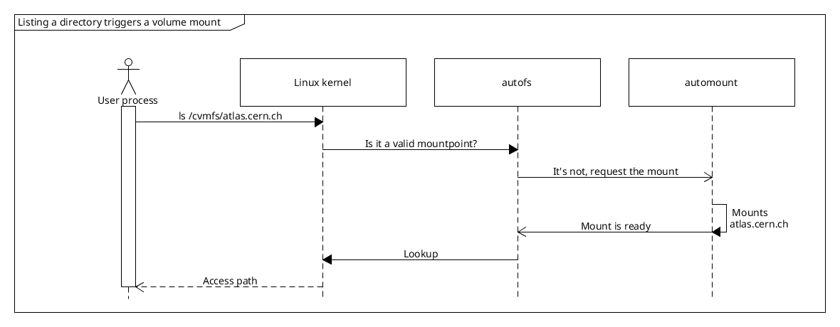
In summary, this is how cvmfs-csi initializes /cvmfs:
- A dedicated container in the Node plugin Pod runs
automount --foreground. With the process running in foreground it’s much easier to control its lifetime and capture its logs. - It waits until
/cvmfsis an autofs mountpoint (filesystem type0x0187). - It makes the autofs root shared with
mount --make-shared /cvmfs.
Node plugin needs to be run with hostPID: true, otherwise mount requests are not reaching the daemon:
# Running commands on the host node:

# * /var/cvmfs is the autofs root mountpoint (hostPath exposed to the Node plugin Pod).
# * The automount container runs in its own PID namespace.
# * Accessing /var/cvmfs/atlas.cern.ch does not trigger a mount in the automount daemon.
[root@rvasek-1-27-6-2-qqbsjsnaopix-node-0 /]# ls /var/cvmfs
[root@rvasek-1-27-6-2-qqbsjsnaopix-node-0 /]# ls /var/cvmfs/atlas.cern.ch
ls: cannot access '/var/cvmfs/atlas.cern.ch': No such file or directory

# Now, running automount in host's PID namespace.
[root@rvasek-1-27-6-2-qqbsjsnaopix-node-0 /]# ls /var/cvmfs/atlas.cern.ch
repo
Next, let’s see how we expose the autofs root to other Pods, in the context of a CSI Node plugin. Under the hood it’s all just bindmounts and mount sharing.
Sharing is caring, unless…
Let’s have a Pod that mounts a CVMFS PersistentVolume. As it gets scheduled on a node, kubelet invokes NodePublishVolume RPC on the cvmfs-csi Node plugin. The RPC’s request contains target_path: a hostPath where kubelet expects a new volume mount to appear, so that it can bind-mount it into the container that’s about to be started. This is where we expose the autofs root.
/cvmfs is made ready during Node plugin’s initialization (see above), so when a consumer Pod comes to the node, NodePublishVolume only needs to bind-mount the autofs root into the target_path:
mount --rbind --make-slave /cvmfs <Request.target_path>
-
--rbind: We use recursive mode because/cvmfsmay already contain mounts. Such situation is very common actually: first consumer Pod accesses/cvmfs/atlas.cern.ch; all consumers that come after must bindmount the inner mounts too. Otherwise they would show up only as empty directories, not being able to trigger autofs to mount them (because from automount’s point-of-view, the path and the mount already exists). -
--make-slave: We maketarget_patha one-way shared bindmount. There are a couple of reasons why it needs to be configured like that.By default, mountpoints are private. As such, one of the consequences is that if a new mount appears under the path, any later bindmounts of the path will not receive any (un)mount events. We need the mounts to be propagated though, otherwise if a Pod triggers a mount, it will not be able to access it.
Sharing the mountpoint both ways (with
--make-shared) would make events propagate correctly, and consumer Pods would see new inner mounts appear. But there is a catch: eventually the consumer Pods need to be deleted, triggering unmounts. The same event propagation that made inner mounts visible inside all of the bindmounts now starts working against us. Unmount events would propagate across all the bindmounts, attempting to unmount volumes not only for the Pod that was just deleted, but for all the consumer Pods. Clearly this is not something we want.To limit the blast radius of the events issued by unmounting
Request.target_path, we use slave mounts. They still receive events from the original autofs root, but when they themselves are unmounted, they don’t affect the root – it’s a one-way communication.
We have already touched on consumer Pod deletions and unmounts, but we haven’t described how is it actually done:
umount --recursive <Request.target_path>
--recursive: In general, when a Pod is deleted, its mounts need to be cleaned as well. kubelet invokesNodeUnpublishVolumeRPC on the Node plugin, unmounting the volume. In case of autofs, it’s not enough to justumount <Request.target_path>because the autofs root contains live mounts inside of it (see--rbindabove), and so this would fail withEBUSY. Instead,umount --recursiveneeds to be used.
One last thing to mention regarding unmounts is of course the mount expiry feature. We expose the inactivity timeout via a Helm chart variable, and admins can then configure its value. This didn’t need any specific setup on the CSI driver side, and so we’ll just mention what we’ve observed:
- mount expiry works well. Unmount events are correctly propagated to all slave mounts,
- when a mount expires, the automount daemon calls
umount --lazy, and so the actual unmount is deferred until there is nothing accessing it.
And lastly, consumer Pods need to set up their own mount propagation too, otherwise the events won’t be correctly propagated to the containers. This is easy enough to do:
spec:
  containers:
  - volumeMounts:
    - name: cvmfs
      mountPath: /cvmfs
      mountPropagation: HostToContainer
    ...
This, in short, is all it took to run a basic autofs setup providing mount and unmount support for other Pods on the node. We’ve seen how cvmfs-csi starts the automount daemon, exposes the mountpoint(s) and how the consumers can let go of autofs-managed mounts when they are no longer needed. This all works great. In the next section we’ll describe what happens when the Node plugin Pod is restarted, and how we tackled the issues caused by that.
When things break
Pods can crash, get restarted, evicted. The age-old problem of persisting resources (in this case mounts) in ephemeral containers… If the Node plugin Pod goes down, so will the automount daemon that runs in it.
What can we do about it from within a CSI driver? Articles “Communicating with autofs” and “Miscellaneous Device control operations for the autofs kernel module” at kernel.org discuss autofs restore in great detail, but in short, the daemon must reclaim the ownership of the autofs root in order to be able to handle autofs requests to mount and unmount again. This is something that is supported out-of-the-box, however getting it to work in containers did not go without issues:
- automount daemon cleans up its mounts when exitting,
/dev/autofsmust be accessible,- autofs root must be exposed on the host so that it survives container restarts.
Let’s go through these one by one. We’ve mentioned that the automount daemon needs to be able to reclaim the autofs root. Under normal circumstances, once you ask the daemon to quit, it cleans up after itself and exists as asked. Cleaning up entails unmounting the individual inner mounts, followed up by unmounting the autofs root itself (analogous to umount --recursive /cvmfs). Now, one might ask how is the daemon expected to reclaim anything, if there is no autofs mount anymore?
When the Node plugin Pod is being deleted, kubelet sends SIGTERM to the containers’ main process. As expected, this indeed triggers automount’s mount clean up. This inadvertly breaks the autofs bindmounts in all consumer Pods and what’s worse, there is no way for the consumers to restore access and they all would need to be restarted. There is a way to skip the mount clean up though: instead of the SIGTERM signal, the automount’s container sends SIGKILL to the daemon when shutting down. With this “trick” the autofs mount is kept, and we are able to make the daemon reconnect and serve requests again. Additionally, a small but important detail is that the reconnect itself involves communication with the autofs kernel module via /dev/autofs device, and so it needs to be made available to the Node plugin Pod.
Related to that, the /cvmfs autofs root must be exposed via a hostPath, and be a shared mount (i.e. mount --make-shared, or mountPropagation: Bidirectional inside the Node plugin Pod manifest). Reclaiming the autofs root wouldn’t be possible if the mountpoint was tied to the Node plugin Pod’s lifetime, and so we need to persist it on the host. One thing to look out for is that if there is something periodically scanning mounts on the host (e.g. node-problem-detector, some Prometheus node metrics scrapers, …), it may keep reseting autofs’s mount expiry. In these situations it’s a good idea to exempt the autofs mountpoints from being touched by these components.
Okay, we have the root mountpoint covered, but what about the inner mounts inside /cvmfs? Normally we wouldn’t need to worry about them, but the CVMFS client is FUSE-based filesystem driver, and so it runs in user-space as a regular process. Deleting the Node plugin Pod then shuts down not only the automount daemon, but all the FUSE processes backing the respective CVMFS mounts. This causes a couple of problems:
- (a) losing those FUSE processes will cause I/O errors,
- (b) since we SIGKILL’d automount, the mounts still appear in the mount table and are not cleaned up,
- (c) automount doesn’t recognize the errors reported by severed FUSE mounts (
ENOTCONNerror code) and this prevents mount expiry from taking place.
While we cannot do anything about (a), (c) is the most serious in terms of affecting the consumers: if expiration worked, the severed mounts would be automatically taken down, and eventually mounted again (the next time the path is accessed), effectively restoring them. To work around this, we deploy yet another container in the Node plugin Pod. Its only job is to periodically scan /cvmfs for severed FUSE mounts, and in case it finds any, it unmounts them. To remount it, all it takes is for any consumer Pod on the node to access the respective path, and autofs will take care of the rest.
Conclusion
autofs is not very common in CSI drivers, and so there is not a lot of resources online on this subject. We hope this blogpost sheds a bit more light on the “how” as well as the “why”, and shows that as long as things are set up correctly, automounts indeed work fine in containers. While we have encountered numerous issues, we’ve managed to work around most of them. Also, we are in contact with the upstream autofs community and will be working towards fixing them, improving support for automounts in containers.
Summary check-list:
- Node plugin needs to be run with
hostPID: true - autofs root must be a shared mount in a hostPath
- bindmounting autofs should be done with
mount --rbind --make-slave - unmounting autofs bindmounts should be done with
umount --recursive - Node plugin Pods need access to
/dev/autofs - the automount daemon should be sent SIGKILL when shutting down
Resources:
GitLab Runners and Kubernetes: A Powerful Duo for CI/CD
Introduction
A GitLab runner is an application that works with GitLab CI/CD to run jobs in a pipeline. GitLab at CERN provides runners that are available to the whole instance and any CERN user can access them. In the past, we were providing a fixed amount of Docker runners executing in Openstack virtual machines following an in-house solution that utilized docker machine. This solution served its purpose for several years, but docker machine was deprecated by Docker some years ago, and a fork is only maintained by GitLab. The last few years CERN’s GitLab licensed users have increased and together with them, even more the number of running pipelines, as Continuous Integration and Delivery (CI/CD) is rapidly adopted by everyone. We needed to provide a scalable infrastructure that would facilitate our users’ demand and CERN’s growth and Kubernetes Runners seemed promising.
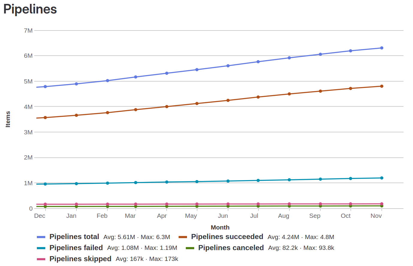
Figure 1: Evolution in the Number of Pipelines over the last year (Dec 2022 – Nov 2023)
Kubernetes+executor Runners: Our new powerful tool
The Kubernetes runners come with the advantages that Kubernetes have in terms of reliability, scalability and availability providing a robust infrastructure for runners to flourish hand by hand with our users’ activities. The new infrastructure has many advantages over the old one. It is safe to say that it suits our needs better as a big organization with a range of activities in research, IT infrastructure and development. Some of the advantages that Kubernetes Runners have are:
- Scalability: Kubernetes runners can scale from 0 to 100 pods at any given time depending on the demand across more than 20 nodes. We can also scale the cluster to any number of nodes to execute 200 jobs concurrently seamlessly, if the demand increases in the future. Here is a time frame in which instance runners went from 0 to 100 jobs in a minute.
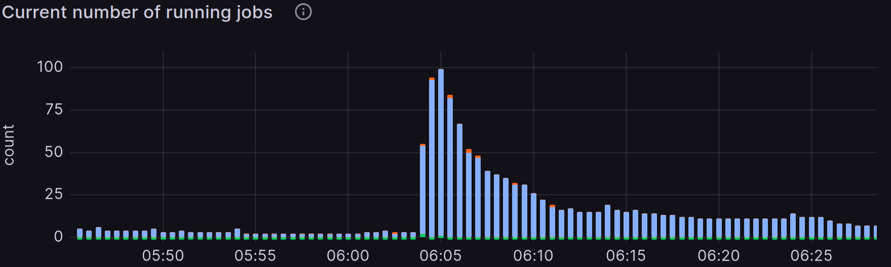
Figure 2: Grafana table of the running jobs in relation to time
Having multiple clusters gives us this advantage multiple times since the jobs are distributed in different specialized clusters depending on the users’ needs.
-
Multi Cluster Support: With multiple clusters, we are able to provide a variety of capabilities to our users based on their needs. Having 19,000 users, physicists, machine learning developers, hardware designers, software engineers means that there is not a silver bullet for shared runners. Hence, it is GitLab’s great responsibility to provide multiple instances to facilitate users’ activities. Those instances are:
- Default cluster: Generic runners that can accommodate the vast majority of jobs.
- CVMFS cluster: CVMFS stands for CernVM File System. It is a scalable, reliable, and low-maintenance software distribution service. It was developed to assist High Energy Physics (HEP) collaborations to deploy software on the worldwide-distributed computing infrastructure used to run data processing applications. The CVMFS Cluster mounts CVMFS volumes per job.
- ARM cluster: For building ARM executables with the advantages that this architecture has such as high performance, energy efficiency, and integrated security.
- FPGA cluster: At CERN, FPGAs are extensively used not only in scientific experiments but also in the operation of accelerators, where they provide specialized circuits tailored for unique applications. To support the development of these FPGA-based systems, CERN’s CI/CD infrastructure includes customized runners designed to handle FPGA development-related jobs.
- Apache Spark cluster: Apache Spark is a general-purpose distributed data processing engine and vastly used at CERN for several data analytics applications regarding research for high energy physics, AI and more.
We also have plans to incorporate new clusters in our toolbox. Those are:
- GPU cluster: Specialized runners to run jobs on GPUs for highly parallelizable workloads to accelerate our applications regarding machine learning and data processing
- Technical Network cluster: An air-gapped deployment offering connectivity for accelerator control devices and accelerator related industrial systems at CERN.
-
Easy Cluster Creation: We used Terraform to create clusters seamlessly for the different types of clusters we use as mentioned earlier. To achieve this, we used the GitLab Integration with Terraform and we are also following up OpenTofu. Furthermore, in case of a severe issue or a compromise of a cluster, we can bring the cluster down and create a new one with very few manual steps. Here is a part of our pipeline that we use to create clusters.
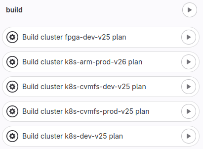
Figure 3: Part of the cluster creation pipeline
Architectural Overview
Let’s take a step back and see the big picture, what decisions we made and why. The following Figure 4 represents the architecture overview of the installation we implemented. The deployment of the runners has been decoupled from the GitLab cluster which has a lot of benefits:
- Cluster decoupling: Previously, the Docker executors were deployed in the same cluster as the GitLab application. Now, the runners have their own clusters which gives the advantage to maintain them separately, organize the infrastructure and runners’ configuration better per environment, and have specific end-to-end tests which allows us to verify their operability without interfering with the GitLab Application.
- Zero downtime Cluster upgrades: With this architecture we can upgrade the runners’ clusters to a more recent Kubernetes version with zero downtime by simply creating a new cluster and then registering it as an instance runner with the same tags, and finally decommissioning the old cluster. When both clusters are simultaneously running, GitLab will balance the jobs between them.
- Scaling-up: GitLab Service has a QA infrastructure to verify and assure the quality of the service before releasing. As such, this instance comes with its own set of runners which can be registered to the production instance at any time, scaling the GitLab infrastructure up to the required demand in an emergency situation.
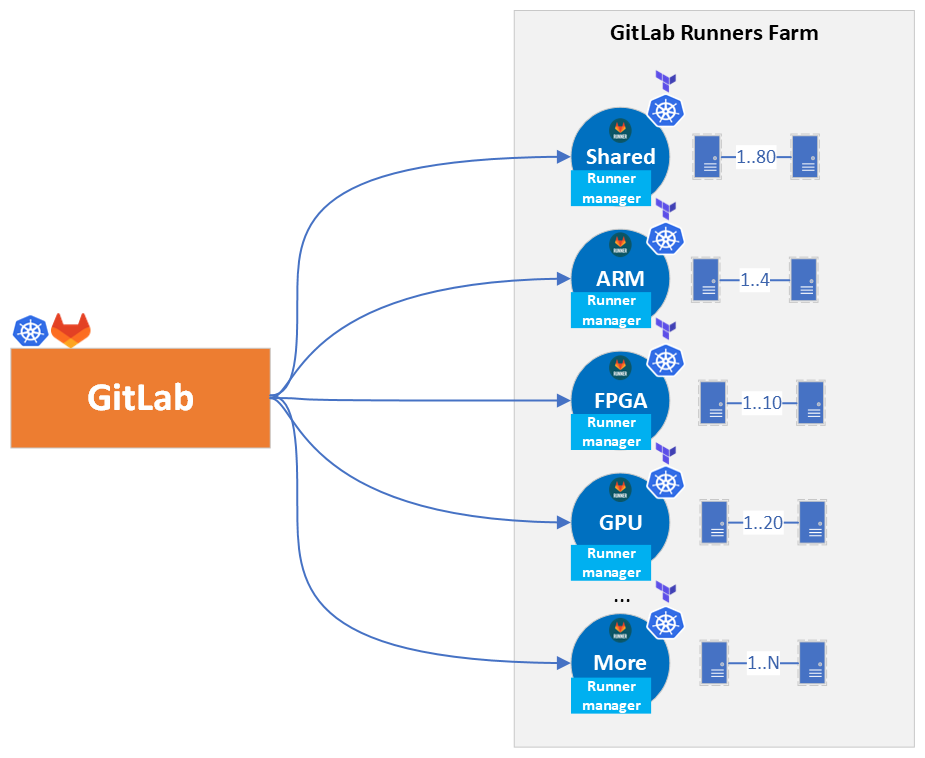
Figure 4: GitLab connection to Runners Architecture Overview
How we migrated to K8s Runners?
In order to migrate to the GitLab runners we performed a series of steps detailed next:
- Creation of a temporary tag (k8s-default)
- Opt-in offering and randomly selection of users to try them out
- Accept untagged jobs
- Finally, decommission Docker runners
Lets see the above in more detail.
![Figure 5: GitLab runners migration tImeline [2023]](/blog/2023/12/06/gitlab-runners-and-kubernetes-a-powerful-duo-for-ci/cd/images/migration-timeline.png)
Figure 5: GitLab runners migration tImeline [2023]
After setting up the clusters and registering them in GitLab, we announced a temporary tag for users interested in using the new runners, named k8s-default. Jobs were running in the new executor successfully without any problems and more and more users opted-in to try our new offering. This certainly helped us troubleshooting GitLab Runners, and start getting acquainted and embracing a very valuable experience and know-how on them.
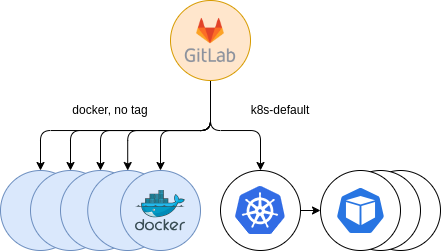
Figure 6: Initial Kubernetes providing. Opt-in
The next step was to gradually accept jobs from untagged jobs. We kept supporting previous Docker runners, in order to provide a fallback mechanism for users that, in the event of starting to use the new Kubernetes runners, experienced some errors. Thus, users using the docker tag in their .gitlab-ci.yml configuration file, would automatically land in the Docker runners, while those with untagged jobs, in addition to the k8s-default tag, started landing in the new Kubernetes runners. This gave us some insights of problems that could occur and to solve them before the full migration.
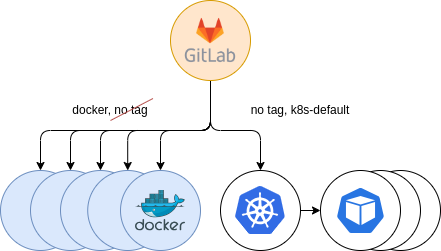
Figure 7: Secondary Kubernetes providing. Parallel to Docker
The last step was to decommission the old runner tags and move everything to the new infrastructure.
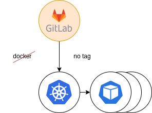
Figure 8: Final providing. Docker decommission
As a result, the Kubernetes runner accepted all the load and users that didn’t migrate to the new runners already had been forced to do it.
Errors and pitfalls
Such a big migration to the new runners had some problems and pitfalls that we discovered as we went through. Several analysis, investigations and communication with users helped us address them, aiming at providing a stable environment for our community. Here are some of the tricky problems we solved:
- Ping: Ping was disabled by default and some jobs were failing. This is caused by the security hardening Kubernetes has which disables all sysctls that may be used to access kernel capabilities of the node and interfere with other pods, including the NET_RAW capability which includes all network sysctls for the pod.
- CVMFS: There was a missing configuration in the Kubernetes configmap that was setting up the mount to the CVMFS file system, but thanks to our colleagues from the Kubernetes Team this has been solved in recent versions of CERN Kubernetes clusters (>=1.26). New clusters will benefit from this improvement.
- IPV6: The new runners are mainly using IPV6 addresses and some users that used IPV4 experienced problems in test cases that run lightweight web servers in, for example, address 127.0.0.1. This is because the pods run their own private network while the Docker runners used the host’s one.
- Entrypoint: The entrypoint in a Docker image is not executed by default due to the recent feature flag introduced in the new GitLab runners based on Kubernetes about honoring (or not) the entrypoint (FF_KUBERNETES_HONOR_ENTRYPOINT). This was not the case for Docker runners, where all runners were executing the entrypoint script in the beginning of the job. It led users into a situation where they hit a limitation, when after honoring the entrypoint of a Dockerfile, this entrypoint contained environment variables defined in the GitLab CI/CD variables. This approach is not valid anymore, and GitLab recommends using/moving the content of this entrypoint to the before_script keyword whenever possible.
- Ulimit Issue: The new Kubernetes cluster we created sets the limit of the file descriptors (ulimit) of the pods that it spawns to the maximum number possible. This is due to a default configuration in the container runtime (in our case, containerd), that in recent versions of Kubernetes, set its limit to
Infinity, the highest possible value. This caused some pods to run really slow and users complained that their jobs, which previously ran in minutes, now hang and after an hour the job was killed. This issue was challenging to address, but it was mainly related to images based on CentOS7, thus needing a lower limit to operate properly, as per this kernel bug. Nevertheless, thanks to the “pre_build_script” setting available in the GitLab Runners configuration, we could “inject” an appropriate ulimit value for all jobs, working around the issue.
Furthermore, we ran into many GitLab bugs that we raised with GitLab’s developers to be assessed, such as an issue that does not allow users to see environment variables in the Terminal or missing documentation that is crucial for customers.
As a result, CERN is becoming a more prominent figure and valued collaborator in the GitLab community through all our contributions and presence.
Security
When we transitioned from Docker runners to Kubernetes runners, it brought a significant improvement in security through the implementation of the UserNamespacesStatelessPodsSupport feature. This feature offered a substantial enhancement to the security of containerized workloads compared to the older Docker setup.
With UserNamespacesStatelessPodsSupport in Kubernetes, we were able to establish a clear separation between containerized applications and the underlying host system by running pods and containers with different user and group IDs than the host system, and by mapping them to different user namespaces. This was a security measure as it mitigated, among others, the risks associated with running containers as the root user on the host system, which could be exploited by malicious actors, potentially leading to the entire system being compromised. The implementation of UserNamespacesStatelessPodsSupport enabled users to effectively isolate containers and their workloads from the host system, thereby enhancing overall system security.
We are committed to the continuous enhancement of our security measures, with a proactive approach to implementing additional safeguards as soon as they become available. For example, it is planned to disable umask 0000 for the Kubernetes runners pods, adopting and going a step further with the security measures and best practices that have been already implemented in docker machine executor runners.
Future Security Hardening
We are actively collaborating with the CERN Security Team to establish comprehensive Security Policies for projects. These security policies are designed to enforce best practices and keep workflows up-to-date. Our collaboration with the CERN Security Team aims to establish a framework that ensures user compliance and promotes a security-conscious culture in our environment. We will talk more about security policies on a separate topic in the near future.
Conclusion and Future plans
Ultimately, with the GitLab Kubernetes runners, we managed to vastly improve the number of concurrent jobs being executed, support different workflows and cut the operational cost of the infrastructure. As we mentioned above, decoupling the clusters speeds up vastly the way we deploy, test and provide the runners, gaining in maintainability aspects.
Our future plans include the provisioning of privileged Kubernetes runners that will set the tombstone in the old docker machine runners and will complete the turnover for Kubernetes runners. It will be challenging, but we are determined to accomplish this following GitLab’s decisions and best practices.
All in all the Git Service is proud of providing our users with an exceptional infrastructure that facilitates the needs of the huge CERN scientific community. We would like to wholeheartedly thank the users that supported us with this improvement and helped us to find out breaking points of the new Kubernetes runners. Together, we managed to stabilize the new runners to be a powerful item in our tool case.
Happy GitLabing to all!
The GitLab Team
Ismael Posada Trobo ismael.posada.trobo@cern.ch
Konstantinos Evangelou konstantinos.evangelou@cern.ch
Subhashis Suara subhashis.suara@cern.ch
Special Thanks to
Ricardo Rocha for his suggestions and support
Nurturing Sustainability: Raising Power Consumption Awareness
Supervisors: Diana Gaponcic, Ricardo Rocha
With modern society relying more and more on digital services this has led to an explosive growth in data centres and cloud-based applications. This growth comes at a cost – data centres are power-hungry and contribute significantly to carbon emissions. To address this, multiple efforts and projects have been looking at integrating sustainability practices in all tech areas, including containers and clusters.
As part of my summer internship with CERN openlab i had the chance to join the CERN Kubernetes team to try out some of these tools, and hopefully launch the first steps to integrate them with the CERN infrastructure.
While having fun, travelling, and making new friends at the same time…
This blog post focuses on finding ways to populate power consumption metrics and visualize them in meaningful ways. It should help raise awareness and find ways to minimize the carbon footprint without compromising application efficiency.
In this blog post, we use Kepler to estimate the power consumption. While this project is obviously a good choice due to its active open-source community, multiple installation ways, and various well-documented metrics, there are some other promising projects in the ecosystem worth trying out.
Kepler Architecture
Kepler (Kubernetes Efficient Power Level Exporter) is an open-source project that uses eBPF to probe CPU performance counters and Linux kernel tracepoints. This data can then be put against actual energy consumption readings or fed to a machine learning model to estimate energy consumption, especially when working with VMs where this information is not available from the hypervisor. The metrics are exported to Prometheus and can be integrated as part of the monitoring. An overview of the architecture can be seen below:

Source: github.com/sustainable-computing-io/kepler-model-server
Kepler Exporter
The Kepler Exporter is a crucial component responsible for exposing the metrics related to energy consumption from different Kubernetes components like Pods and Nodes.

Source: github.com/sustainable-computing-io/kepler
- The Kepler Exporter collects energy consumption metrics from Kubernetes components such as Pods and Nodes using eBPF.
- The metrics are available in Prometheus and be be visualized with Grafana.
- Later, the metrics could be utilized to make scheduling decisions to optimeze the power consumption.
To find more about eBPF in Kepler consult the documentation.
Kepler Model Server
The Kepler Model Server plays a central role in the Kepler architecture. It is designed to provide power estimation models based on various parameters and requests. These models estimate power consumption based on factors like target granularity, available input metrics, and model filters.
- The Kepler Model Server receives requests from clients, which include details about the target granularity (e.g., node, pod), available input metrics, and model filters.
- Based on these requests, the server selects an appropriate power estimation model.
- The Kepler Estimator, which is a client module, interacts with the Kepler Model Server as a sidecar of the Kepler Exporter’s main container. It serves PowerRequests by utilizing the model package defined in Kepler Exporter’s estimator.go file via a unix domain socket.
There is also the possibility of deploying an online-trainer. It runs as a sidecar to the main server, and executes training pipelines to update the power estimation model in real-time when new power metrics become available.
Kepler Estimator
The Kepler Estimator serves as a client module to the Kepler Model Server, running as a sidecar of the Kepler Exporter’s main container. It handles PowerRequests and interacts with the power estimation models to provide power consumption estimates.
- The Kepler Estimator acts as a client module to the Kepler Model Server.
- It receives PowerRequests from the model package in the Kepler Exporter via a unix domain socket (/tmp/estimator.sock).
- The Kepler Estimator uses the power estimation models available in the Kepler Model Server to calculate power consumption estimates based on the provided parameters.
- These estimates are then available to the Kepler Exporter.
Installation
The project was designed to be easily installed, and provides multiple ways to do so:
- using an existing helm chart
- building manifests with make
- using the Kepler operator
We tried all installation options. While all methods should work out of the box, we encountered a few issues and settled on building the manifests using make. The command used is:
make build-manifest OPTS="PROMETHEUS_DEPLOY ESTIMATOR_SIDECAR_DEPLOY MODEL_SERVER_DEPLOY"
More configuration options can be found in the documentation.
Running the command above and applying the resulting manifests deploys an exporter (with the estimator as a sidecar) on each node, and the model server:
$ kubectl get pod -n kepler
NAME                                   READY   STATUS    RESTARTS   AGE
kepler-exporter-8t6tb                  2/2     Running   0          18h
kepler-exporter-bsmmj                  2/2     Running   0          18h
kepler-exporter-k4dtb                  2/2     Running   0          18h
kepler-model-server-68df498948-zfblr   1/1     Running   0          19h
Kepler projects provides a Grafana dashboard to visualize the metrics.
While the pods were running successfully, no data was available in Prometheus. This lead to some further investigations.
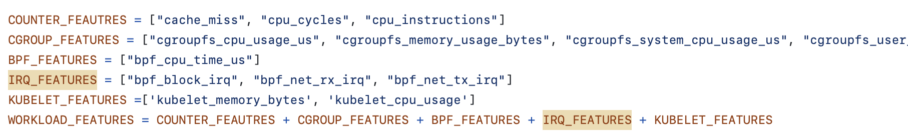
Issue 1: different number of headers and values in the request
The Kepler Estimator module receives a request from the exporter similar to:
"cpu_time","irq_net_tx","irq_net_rx","irq_block","cgroupfs_memory_usage_bytes",
"cgroupfs_kernel_memory_usage_bytes","cgroupfs_tcp_memory_usage_bytes","cgroupfs_cpu_usage_us",
"cgroupfs_system_cpu_usage_us","cgroupfs_user_cpu_usage_us","cgroupfs_ioread_bytes",
"cgroupfs_iowrite_bytes","block_devices_used","container_cpu_usage_seconds_total",
"container_memory_working_set_bytes","block_devices_used"],"values":[[0,0,0,0,0,0,0,0,0,0,0,0,0,0,0],
[0,0,0,0,0,0,0,0,0,0,0,0,0,0,0]],"output_type":"DynComponentPower","system_features":["cpu_architecture"],
"system_values":["Broadwell"],"model_name":"","filter":""}
The request above will error with: {'powers': [], 'msg': 'fail to handle request: 16 columns passed, passed data had 15 columns'}.
For some reason block_devices_used appears twice in the headers. After some investigation, we just added a check that examines the length of the header array and eliminates the last occurrence of “block_devices_used”. This issue needs further investigation.
Issue 2: IRQ metrics naming convention
In the Kepler Estimator request, the IRQ metrics have irq- at the beginning: irq_net_tx, irq_net_rx, and irq_block. At the same time, in the Kepler Model Server, -irq is placed at the end of the name.
Compare:
- In Kepler Estimator:
"cpu_time","irq_net_tx","irq_net_rx","irq_block","cgroupfs_memory_usage_bytes"... - In Kepler model server:
This missmatch prevents the model server from returning a model, because of the missing features:
valid feature groups:  []
DynComponentPower
10.100.205.40 - - [18/Aug/2023 12:09:44] "POST /model HTTP/1.1" 400 -
To address the problem, an upstream issue was opened. The community was remarkably responsive, validating the problem and coming up with a fix.
Demo Time
Create some test load
After deploying Kepler and resolving the issues above, we can proceed and create some stress load using a tool called stress-ng. It is important to limit the memory the pod can utilize, to avoid other pods being killed.
apiVersion: v1
kind: Pod
metadata:
 name: stress-ng
 namespace: kepler
spec:
 containers:
  - name: stress-ng
    image: polinux/stress-ng
    command: ["sleep","inf"]
    resources:
      requests:
        memory: "1.2G"
      limits:
        memory: "1.2G"
Some commands that were utilized in the analysis:
stress-ng --cpu 4 --io 2 --vm 1 --vm-bytes 1G --timeout 30sstress-ng --disk 2 --timeout 60s --metrics-briefstress-ng --cpu 10 --io 2 --vm 10 --vm-bytes 1G --timeout 10m --metrics-brief
For more available parameters consult the relevant documentation.
Analyzing the Results
Access Grafana Kepler dashboard and monitor the metrics when creating the test load. We can clearly see the spikes in power consumption:
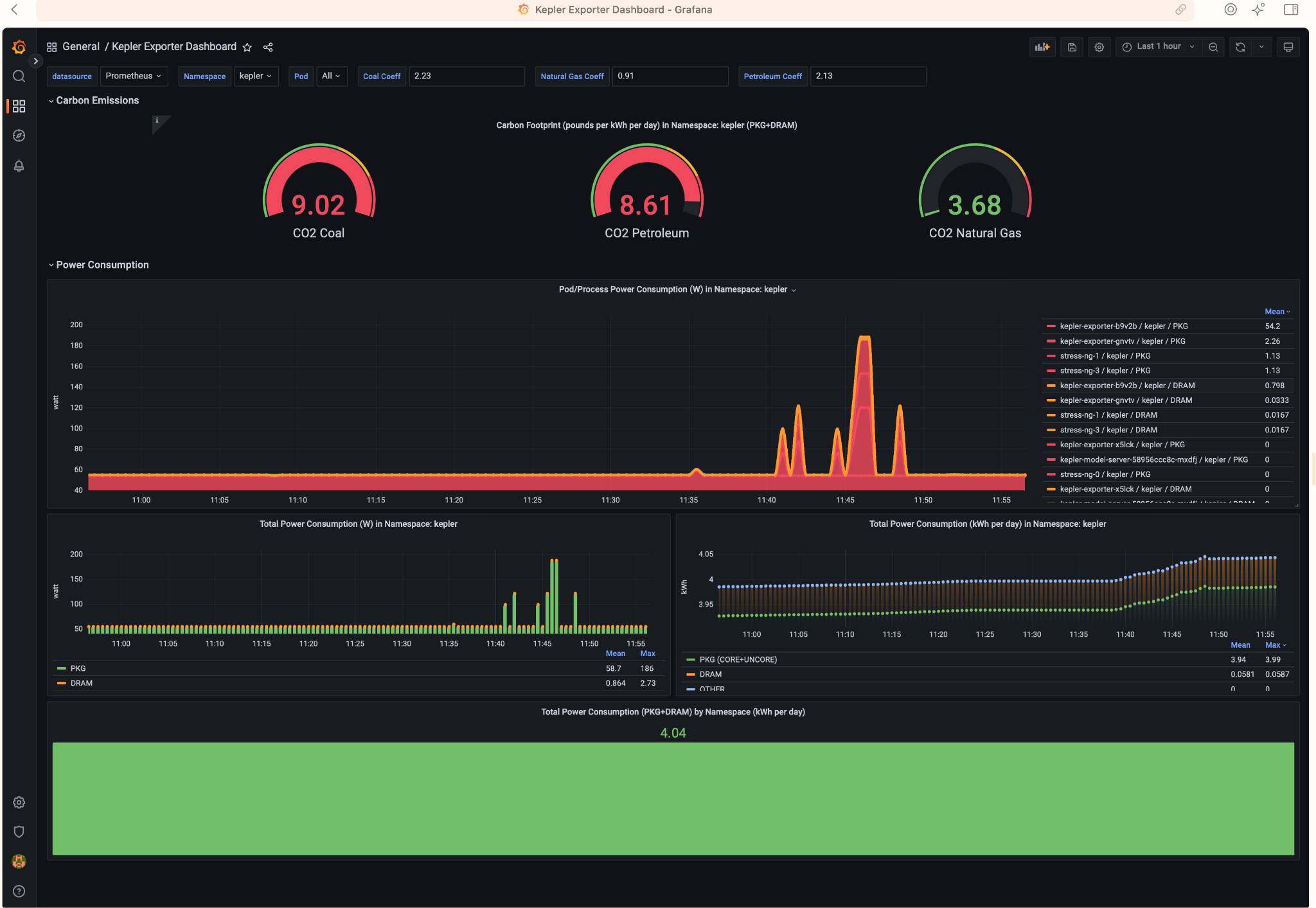
We can monitor the power consumption per process/pod. For example If we choose only the stress-ng pod:
A panel worth to mention is “Carbon Footprint in Namespace”, where the metrics can be combined with power usage effectiveness (PUE) and electricity carbon intensity data to calculate the carbon footprint of the workload:
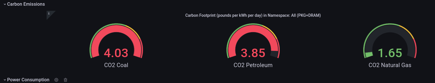
By observing resource utilisation and energy consumption at pod- and node- level we can better understand the environmental impact of a running Kubernetes cluster. Using data analysis we can make better decisions on how to allocate resources, optimize our workloads and architect our applications.
Conclusion and Future work
Engaging in a summer project focused on platform-aware scheduling using the Kepler library has proven to be a highly productive and valuable endeavor. This project has brought to light the substantial correlation between technology and environmental sustainability by exploring energy consumption metrics and carbon footprint data within Kubernetes clusters, both at the node and pod levels. Some future directions to take:
- To look into power aware scheduling:
While having fun, travelling, and making new friends at the same time…
Efficient Access to Shared GPU Resources: Part 6
As the sixth blog post in our series, we are bringing a story about training a high energy physics (HEP) neural network using NVIDIA A100 GPUs using Kubeflow training operators. We will go over our methodology and analyze the impact of various factors on the performance.
This series focuses on NVIDIA cards, although similar mechanisms might be offered by other vendors.
Motivation
Training large-scale deep learning models requires significant computational power. As models grow in size and complexity, efficient training using a single GPU is often not a possibility. To achieve efficient training benefiting from data parallelism or model paralellism, access to multiple GPUs is a prerequisite.
In this context, we will analyze the performance improvements and communication overhead when increasing the number of GPUs, and experiment with different topologies.
From another point of view, as discussed in the previous blog post, sometimes it is beneficial to enable GPU sharing. For example, to have a bigger GPU offering or ensure better GPU utilization. In this regard, we’ll experiment with various A100 MIG configuration options to see how they affect the distributed training performance.
We are aware that training on partitioned GPUs is an unusual setup for distributed training, and it makes more sense to give direct access to full GPUs. But given a setup where the cards are already partitioned to increase the GPU offering, we would like to explore how viable it is to use medium-sized MIGs instances for large training jobs.
Physics Workload - Generative Adversarial Network (GAN)
The computationally intensive HEP model chosen for this exercise is a GAN for producing hadronic showers in the calorimeter detectors. This neural network requires approximately 9GB of memory per worker and is an excellent demonstration of the benefits of distributed training. The model is implemented by Engin Eren, from DESY Institute. All work is available in this repository.
GANs have shown to enable fast simulation in HEP vs the traditional Monte Carlo methods - in some cases this can be several orders of magnitude. When GANs are used, the computational load is shifted from the inference to the training phase. Working efficiently with GANs necessitates the use of multiple GPUs and distributed training.
Setup
The setup for this training includes 10 nodes each having 4 A100 40GB PCIe GPUs, resulting in 40 available GPU cards.
When it comes to using GPUs on Kubernetes clusters, the GPU operator is doing the heavy lifting - details on drivers setup, configuration, etc are in a previous blog post.
Training deep learning models using Kubeflow training operators requires developing the distributed training script, building the docker image, and writing the corresponding yaml files to run with the proper training parameters.
Developing a distributed training script
- TensorFlow and PyTorch offer support for distributed training.
- Scalability should be kept in mind when creating an initial modelling script. This means introducing distribution strategies and performing data loading in parallel. Starting the project in this manner will make things easier further down the road.
Building a Docker image with dependencies
- Consult the Dockerfile used for this analysis for more information.
- Kubeflow makes use of Kubernetes, a container orchestrator, which means that the distributed training will be run as a group of containers running in parallel and synchronizing with one another.
Creating a yaml file defining training parameters
- Training parameters include image name, the command to run, volume and network file system access, number of workers, number of GPUs in each worker, etc.
- Check the GAN PyTorchJob file used for more information.
The distributed training strategy used for training the GAN for producing hadronic showers in the calorimeter detectors is DistributedDataParallel from PyTorch, which provides data parallelism by synchronizing gradients across each model replica.
Training Time
Let’s start by training the model on 4, 8, 16, and 32 A100 40GB GPUs and compare the results.
| Number of GPUs | Batch Size | Time per Epoch [s] |
|---|---|---|
| 4 | 64 | 210 |
| 8 | 64 | 160 |
| 16 | 64 | 120 |
| 32 | 64 | 78 |
Ideally, when doubling the number of GPUs, we would like to have double the performance. In reality the extra overhead smooths out the performance gain:
| T(4 GPUs) / T(8 GPUs) | T(8 GPUs) / T(16 GPUs) | T(16 GPUs) / T(32 GPUs) |
|---|---|---|
| 1.31 | 1.33 | 1.53 |
Conclusions:
- As expected, as we increase the number of GPUs the time per epoch decreases.
- As we double the number of GPUs, the 30% improvement achieved is lower than expected. This can be caused by multiple things, but one viable option to consider is using a different framework for distributed training. Examples include DeepSpeed or FSDP.
Bringing MIG into the mixture
Next, we can try and perform the same training on MIG-enabled GPUs. In the measurements that follow:
mig-2g.10gb- every GPU is partitioned into 3 instances of 2 compute units and 10 GB virtual memory each (3*2g.10gb).mig-3g.20gb- every GPU is partitioned into 2 instances of 3 compute units and 20 GB virtual memory each (2*3g.20gb).
For more information about MIG profiles check the previous blog post and the upstream NVIDIA documentation. Now we can redo the benchmarking, keeping in mind that:
- The mig-2g.10gb configuration has 3 workers per GPU, and mig-3g.20gb has 2 workers.
- On more powerful instances we can opt for bigger batch sizes to get the best performance.
- There should be no network overhead for MIG devices on the same GPUs.
2g.10gb MIG workers
| Number of A100 GPUs | Number of 2g.10gb MIG instances | Batch Size | Time per Epoch [s] |
|---|---|---|---|
| 4 | 12 | 32 | 505 |
| 8 | 24 | 32 | 286 |
| 16 | 48 | 32 | 250 |
| 32 | 96 | 32 | OOM |
The performance comparison when doubling the number of GPUs:
| T(12 MIG instances) / T(24 MIG instances) | T(24 MIG instances) / T(48 MIG instances) | T(48 MIG instances) / T(96 MIG instances) |
|---|---|---|
| 1.76 | 1.144 | OOM |
Conclusions:
- Huge improvements when scaling from 4 to 8 GPUs, the epoch time decreased from 505 to 286 seconds, about 76%.
- Doubling the number the GPUs again (from 8 to 16) improved the time by only ~14%.
- When fragmenting the training too much, we can encounter OOM errors.
- As we use DistributedDataParallel from PyTorch for data parallelism, the OOM is most likely caused by the extra memory needed to do gradient aggregation.
- It can also be caused by inefficiencies when performing the gradient aggregation, but nccl (the backend used) should be efficient enough. This is something to be investigated later.
3g.20gb MIG workers
| Number of full A100 GPUs | Number of 3g.20gb MIG instances | Batch Size | Time per Epoch [s] |
|---|---|---|---|
| 4 | 8 | 64 | 317 |
| 8 | 16 | 64 | 206 |
| 16 | 32 | 64 | 139 |
| 32 | 64 | 64 | 114 |
The performance comparison when doubling the number of GPUs:
| T(8 MIG instances) / T(16 MIG instances) | T(16 MIG instances) / T(32 MIG instances) | T(32 MIG instances) / T(64 MIG instances) |
|---|---|---|
| 1.53 | 1.48 | 1.21 |
Conclusions:
- When increasing the number of GPUs from 4 to 8, initially the scaling is less aggressive than it was for 2g.10gb instances (53% vs 76%), but it is more stable and allows to further increase the number of GPUs.
mig-3g.20gb vs mig-disabled:
There are some initial assumptions we have, that should lead to the mig-disabled setup being more efficient than mig-3g.20gb. Consult the previous blogpost for more context:
- Double the number of Graphical Instances:
- In the mig-3g.20gb setup, every GPU is partitioned into 2, as a result, we have double the number of GPU instances.
- This results in more overhead.
- The number of SMs:
- For NVIDIA A100 40GB GPU, 1 SM means 64 CUDA Cores and 4 Tensor Cores
- A full A100 GPU has 108 SMs.
- 2 * 3g.20gb mig instances have in total 84 SMs (3g.20gb=42 SMs, consult the previous blog post for more information).
- mig-disabled setup has 22.22% more CUDA cores and Tensor Cores than mig-3g.20gb setup
- Memory:
- The full A100 GPU has 40GB of virtual memory
- 2 * 3g.20gb mig instances have 2 * 20 GB = 40 GB
- no loss of memory
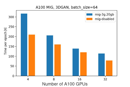
Based on the experimental data, as expected, performing the training on full A100 GPUs shows better results than on mig-enabled ones. This can caused by multiple factors:
- Loss of SMs when enabling MIG
- Communication overhead
- Gradient synchronization
- Network congestion, etc.
At the same time, the trend seems to point out that as we increase the number of GPUs, the difference between mig-disabled vs mig-enabled setup alleviates.
Conclusions
- Although partitioning GPUs can be beneficial for providing bigger GPU offering and better utilization, it is still worth it to have dedicated GPUs for running demanding production jobs.
- Given a setup where GPUs are available but mig-partitioned, distributed training is a viable option:
- It comes with a penalty for the extra communication/bigger number of GPUs to provide same amount of resources.
- Adding small GPU instances can initially speed up the execution, but the improvement will decrease as more overhead is added, and in some cases the GPU will go OOM.
During these tests, we discovered that the training time per epoch varied significantly for the same input parameters (number of workers, batch size, MIG configuration). It led to the topology analysis that follows in the next section.
Topology
Getting variable execution times for fixed inputs lead to some additional investigations. The question is: “Does the topology affect the performance in a visible way?”.
In the following analysis, we have 8 nodes, each having 4 A100 GPUs. Given that we need 16 GPUs for model training, would it be better and more consistent if the workers utilized all 4 GPUs on 4 machines, or if the workers were distributed across more nodes?
To represent topologies, we will use a sequence of numbers, showing how many GPUs were in-use on different nodes.
For example, the topologies below can be represented as 3 2 1 1 1 and 0 0 2 1 1 1 3:
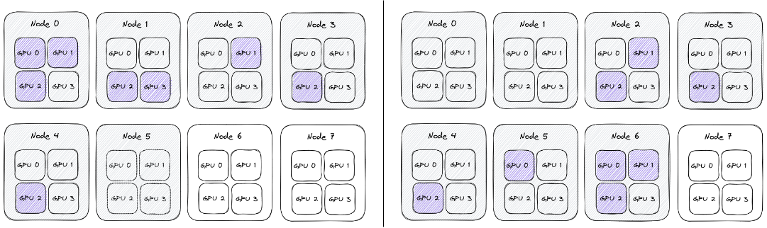
Conceptually all the nodes are the same, and the network behaves uniformly between them, so it shouldn’t matter on which node we schedule the training. As a result the topologies above (0 0 2 1 1 1 3 and 3 2 1 1 1) are actually the same, and can be generically represented as 1 1 1 2 3.
Setup
It seems that when deploying Pytorchjobs, the scheduling is only based on availability of the GPUs. Since there isn’t an automatic way to enforce topology at the node level, the topology was captured using the following procedure:
- Identify schedulable nodes. Begin with four available nodes, then increase to five, six, seven, and eight. Workloads will be assigned to available GPUs by the Kubernetes scheduler. Repeat steps 2 through 5 for each available set of nodes.
- On each GPU, clear memory and delete processes.
- Run a process on each node to monitor GPU utilization (which cards are being used)
- Execute a PyTorchjob with 16 workers.
- Store info about every card utilized from each node and the time of the training job across multiple epochs.
The use case is the same: GAN for producing hadronic showers in the calorimeter detectors, with the batch size of 64. Full A100 GPUs were used for this part, with MIG disabled. The source code for the analysis can be found in this repository.
Analyzing the results
The benchmarking results can be found in the a100_topology_experiment.txt file, but it is pretty hard to make conclusions without visualizing the result.
Each job has three epochs, which are shown in blue, orange, and green. Unfortunately, the number of experiments per topology is not consistent, and can vary from 1 to 20 samples, and at the time of writing the setup cannot be replicated. As a result, take the following observations with a grain of salt.
We try to pinpoint the topologies where the performance is high, but the variance is small. For every topology we have the average excution time, but also how much the value varied across jobs.
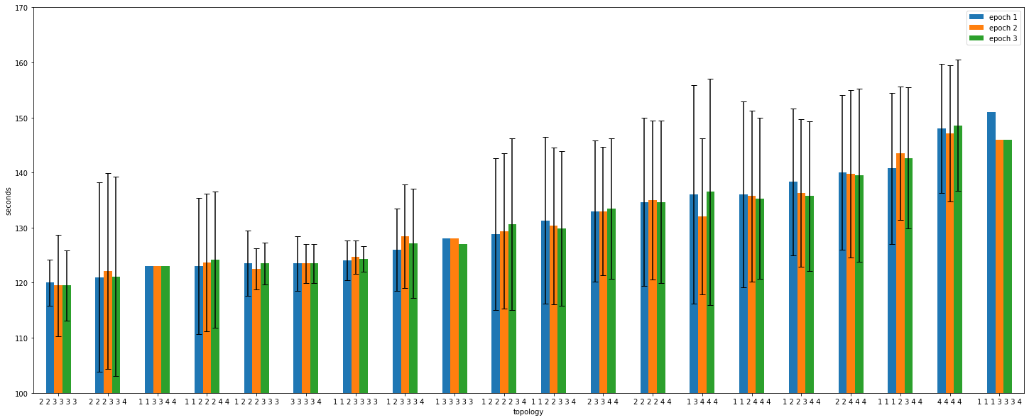
Conclusions
- Even if the topology is fixed, the epoch times vary a lot. For topology
4 4 4 4, the epoch time range from 120 to 160 seconds, even though the whole setup is the same. - The epoch times at the job level do not vary significantly. The main distinction is seen between jobs.
- The best topology is not necessarily the one that produces the best results for a single job, but rather the one that produces the most uniform distribution of results.
- There are some topologies that out-perform others in terms of execution time and stability. By comparing the results it seems that they are skewed towards taking advantage of in-node communication, while leaving resources for bursty behaviour.
- The best results seem to be for
1 2 2 2 3 3 3,3 3 3 3 4, and1 1 2 3 3 3 3topologies. The common point for them is that they take advantage of 3/4 GPUs on the nodes, as a result having fast in-node communication but also making sure there is no GPU congestion.
- The best results seem to be for
This analysis is done at a fairly high level. To gain a better understanding of the performance, we should investigate the NUMA settings. Additionally, different synchronization strategies, such as parameter server, could be used to achieve more consistent performance.
Webinar: Fully Automated Deployments with ArgoCD
The next step after achievement full automated with GitOps for your services and applications is to also apply it to the infrastructure underneath.
Managing multiple clusters can be a challenge, so why not do it in the same way you manage the services running on these clusters? In this webinar we deep dive into a proposal to solve it, taking our 101 ArgoCD tutorial as a starting point.
Efficient Access to Shared GPU Resources: Part 5
This is part 5 of a series of blog posts about GPU concurrency mechanisms. In part 1 we focused on the pros and cons of different solutions available on Kubernetes, in part 2 we dove into the setup and configuration details, in part 3 we analyzed the benchmarking use cases, and in part 4 we benchmarked the time slicing mechanism.
In this part 5 we will focus on benchmarking MIG (Multi-Instance GPU) performance of NVIDIA cards.
This series focuses on NVIDIA cards, although similar mechanisms might be offered by other vendors.
Setup
The benchmark setup will be the same for every use case:
- Full GPU (MIG disabled) vs MIG enabled (7g.40gb partition)
- MIG enabled, different partitions:
- 7g.40gb
- 3g.20gb
- 2g.10gb
- 1g.5gb
Keep in mind that the nvidia-smi command will not return the GPU utilization if MIG is enabled. This is the expected behaviour, as NVML (NVIDIA management library) does not support attribution of utilization metrics to MIG devices. For monitoring MIG capable GPUs it is recommended to rely on NVIDIA DCGM instead.
Find more about the drivers installation, MIG configuration, and environment setup.
Theoretical MIG performance penalty
When sharing a GPU between multiple processes using time slicing, there is a performance loss caused by the context switching. As a result, when enabling time slicing but scheduling a single process on the GPU, the penalty can be neglected.
On the other hand, with MIG, the assumptions are very different. By just enabling MIG, a part of the Streaming Multiprocessors are lost. But there is no additional penalty introduced when further partitioning the GPU.
For instance, as can be seen in the image below, a whole A100 40GB NVIDIA GPU (the GPU used for the benchmarking that follows) has 108 Streaming Multiprocessors (SMs). When enabling MIG, 10 SMs are lost, which is the equivalent of 9.25% of the total number of compute cores.
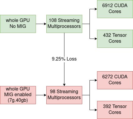
As a result, when enabling MIG, it is expected to see a performance penalty of ~9.25%. As partitions are considered isolated, we shouldn’t have additional overhead when sharing the GPU between many users. We expect the scaling between partitions to be linear, meaning a 2g.10gb partition should perform 2 times better than a 1g.5gb because it has double the resources.
FLOPS Counting
Floating Point Operations Per Second (FLOPS) is the metric used to show how powerful a GPU is when working with different data formats. To count FLOPS we rely on dcgmproftester, a CUDA-based test load generator from NVIDIA. For more information, consult the previous blog post.
Full GPU (MIG disabled) vs MIG enabled (7g.40gb partition)
| Formats | Full GPU (MIG disabled) [TFLOPS] | MIG enabled (7g.40gb) [TFLOPS] | Loss [%] |
|---|---|---|---|
| fp16, Cuda Cores | 32.785 | 30.583 | 6.71 |
| fp32, Cuda Cores | 16.773 | 15.312 | 8.71 |
| fp64, Cuda Cores | 8.128 | 7.386 | 9.12 |
| fp16, Tensor Cores | 164.373 | 151.701 | 7.70 |
FLOPS counting per MIG partition
| Formats | 7g.40gb [TFLOPS] | 3g.20gb [TFLOPS] | 2g.10gb [TFLOPS] | 1g.5gb [TFLOPS] | |
|---|---|---|---|---|---|
| fp16, Cuda Cores | 30.583 | 13.714 | 9.135 | 4.348 | |
| fp32, Cuda Cores | 15.312 | 6.682 | 4.418 | 2.132 | |
| fp64, Cuda Cores | 7.386 | 3.332 | 2.206 | 1.056 | |
| fp16, Tensor Cores | 151.701 | 94.197 | 65.968 | 30.108 |
FLOPS scaling between MIG partitions
| Formats | 7g.40gb / 3g.20gb | 3g.20gb / 2g.10gb | 2g.10gb / 1g.5gb |
|---|---|---|---|
| fp16, Cuda Cores | 2.23 | 1.50 | 2.10 |
| fp32, Cuda Cores | 2.29 | 1.51 | 2.07 |
| fp64, Cuda Cores | 2.21 | 1.51 | 2.08 |
| fp16, Tensor Cores | 1.61 | 1.42 | 2.19 |
| Ideal Scale | 7/3=2.33 | 3/2=1.5 | 2/1=2 |
Memory bandwidth scaling between MIG partitions
| Partition | Memory bandwidth | Multiplying factor |
|---|---|---|
| 7g.40gb | 1555.2 GB | 8 |
| 3g.20gb | 777.6 GB | 4 |
| 2g.10gb | 388.8 GB | 2 |
| 1g.5gb | 194.4 GB | 1 |
Conclusions
- Enabling MIG:
- For fp32 and fp64, Cuda Cores, the drop in performance is close to the theoretical one.
- For fp16 on Cuda Cores and Tensor Cores, the loss is much smaller than the expected value. Might need further investigation.
- There is no loss of memory bandwidth.
- The scaling between partitions:
- On CUDA Cores (fp16, fp32, fp64) the scaling is converging to the theoretical value.
- On Tensor Cores the scaling diverges a lot from the expected one (especially when comparing 7g.40gb and 3g.20gb). Might need further investigation.
- The scaling of the memory bandwidth is based on powers of 2 (1, 2, 4, and 8 accordingly).
Compute-Intensive Particle Simulation
An important part of CERN computing is dedicated to simulation. These are compute-intensive operations that can significantly benefit from GPU usage. For this benchmarking, we rely on the lhc simpletrack simulation. For more information, consult the previous blog post.
Full GPU (MIG disabled) vs MIG enabled (7g.40gb partition)
| Number of particles | Full GPU (MIG disabled) [seconds] | MIG enabled (7g.40gb) [seconds] | Loss [%] |
|---|---|---|---|
| 5 000 000 | 26.365 | 28.732 | 8.97 |
| 10 000 000 | 51.135 | 55.930 | 9.37 |
| 15 000 000 | 76.374 | 83.184 | 8.91 |
Running simulation on different MIG partitions
| Number of particles | 7g.40gb [seconds] | 3g.20gb [seconds] | 2g.10gb [seconds] | 1g.5gb [seconds] | |
|---|---|---|---|---|---|
| 5 000 000 | 28.732 | 62.268 | 92.394 | 182.32 | |
| 10 000 000 | 55.930 | 122.864 | 183.01 | 362.10 | |
| 15 000 000 | 83.184 | 183.688 | 273.700 | 542.300 |
Scaling between MIG partitions
| Number of particles | 3g.20gb / 7g.40gb | 2g.10gb / 3g.20gb | 1g.5gb / 2g.10gb |
|---|---|---|---|
| 5 000 000 | 2.16 | 1.48 | 1.97 |
| 10 000 000 | 2.19 | 1.48 | 1.97 |
| 15 000 000 | 2.20 | 1.49 | 1.98 |
| Ideal Scale | 7/3=2.33 | 3/2=1.5 | 2/1=2 |
Conclusions
- The performance loss when enabling MIG is very close to the theoretical 9.25%.
- The scaling between partitions converges to the ideal values.
- The results are very close to the theoretical assumptions because the benchmarked script is very compute-intensive, without many memory accesses, being CPU bound, etc.
Machine Learning Training
For benchmarking, we will use a pre-trained model and fine-tune it with PyTorch. To maximize GPU utilization, make sure the script is not CPU-bound, by increasing the number of data loader workers and batch size. More details can be found in the previous blog post.
Full GPU (MIG disabled) vs MIG enabled (7g.40gb partition)
- dataloader_num_workers=8
- per_device_train_batch_size=48
- per_device_eval_batch_size=48
| Dataset size | Full GPU (MIG disabled) [seconds] | MIG enabled (7g.40gb) [seconds] | Loss [%] |
|---|---|---|---|
| 2 000 | 63.30 | 65.77 | 3.90 |
| 5 000 | 152.91 | 157.86 | 3.23 |
| 10 000 | 303.95 | 313.22 | 3.04 |
| 15 000 | 602.70 | 622.24 | 3.24 |
7g.40gb vs 3g.20gb
- per_device_train_batch_size=24
- per_device_eval_batch_size=24
- dataloader_num_workers=4
| Dataset size | 7g.40gb [seconds] | 3g.20gb [seconds] | 3g.20gb / 7g.40gb (Expected 7/3=2.33) |
|---|---|---|---|
| 2 000 | 67.1968 | 119.4738 | 1.77 |
| 5 000 | 334.2252 | 609.2308 | 1.82 |
| 10 000 | 334.2252 | 609.2308 | 1.82 |
When comparing a 7g.40gb instance vs a 3g.20gb one, the amount of cores becomes 2.33 (7/3) times smaller. This is the scale we are expecting to see experimentally as well, but the results are converging to 1.8 rather than 2.3. For machine learning training, the results are influenced a lot by the available memory, bandwidth, how the data is stored, how efficient the data loader is, etc.
To simplify the benchmarking, we will use the 4g.20gb partition instead of the 3g.20gb. This way all the resources (bandwidth, cuda cores, tensor cores, memory) are double when compared to 2g.10gb, and the ideal scaling factor is 2.
4g.20gb vs 2g.10gb:
- per_device_train_batch_size=12
- per_device_eval_batch_size=12
- dataloader_num_workers=4
| Dataset size | 4g.20gb [seconds] | 2g.10gb [seconds] | 2g.10gb / 4g.20gb (Expected 4/2=2) |
|---|---|---|---|
| 2 000 | 119.2099 | 223.188 | 1.87 |
| 5 000 | 294.6218 | 556.4449 | 1.88 |
| 10 000 | 589.0617 | 1112.927 | 1.88 |
2g.10gb vs 1g.5gb:
- per_device_train_batch_size=4
- per_device_eval_batch_size=4
- dataloader_num_workers=2
| Dataset size | 2g.10gb [seconds] | 1g.5gb [seconds] | 1g.5gb / 2g.10gb (Expected 2/1=2) |
|---|---|---|---|
| 2 000 | 271.6612 | 525.9507 | 1.93 |
| 5 000 | 676.3226 | 1316.2178 | 1.94 |
| 10 000 | 1356.9108 | 2625.1624 | 1.93 |
Conclusions
- The performance loss when enabling MIG is much smaller than the theoretical 9.25%. This can be caused by many reasons:
- complex operations to be performed
- being IO bound
- executing at a different clock frequency
- variable tensor core utilization, etc.
- The training time depends heavily on the number of CUDA Cores, Tensor Cores, but also the memory bandwidth, the data loader, the batch size, etc. Consult the previous blog for some ideas on how to profile and detect performance bottlenecks of models.
- The scaling between partitions is linear and is converging to the expected value. Especially on smaller partitions.
Takeaways
- When using MIG technology, the GPU partitions are isolated and can run securely without influencing each other.
- A part of the available streaming multiprocessors are lost when enabling MIG:
- In the case of an A100 40GB NVIDIA GPU, 10/108 SMs, which means losing 9.25% of the available Cuda and Tensor cores.
- Never enable MIG without actually partitioning the GPU (the 7g.40gb partition). It means losing performance without gaining GPU sharing.
- When enabling MIG:
- The performance loss for compute-intensive applications can reach ~9.25%.
- For machine learning training the loss alleviates as a result of memory accessing, being IO bound, being CPU bound, etc, and experimentally it will be much smaller than expected.
- The scaling between partitions is linear. Doubling the resources halves the execution time.
- For GPU monitoring rely on NVIDIA Data Center GPU Manager (DCGM). It is a suite of tools that includes active health monitoring, diagnostics, power and clock management, etc.
- A current limitation (with CUDA 11/R450 and CUDA 12/R525) that might be relaxed in the future is that regardless of how many MIG devices are created (or made available to a container), a single CUDA process can only enumerate a single MIG device. The implications are:
- We cannot use 2 MIG instances in a single process.
- If at least one device is in MIG mode, CUDA will not see the non-MIG GPUs.
Next episode
In the next blog post, we will use NVIDIA A100 GPUs and MIG to train in distributed mode a high energy physics (HEP) neural network on-prem Kubeflow. Stay tuned!
Webinar: Container Storage Improved: What's New in CVMFS and EOS Integrations
We’ve been working hard on improving storage integration with our Kubernetes service offerings.
This webinar is a great opportunity to catch up with all the latest improvements, including better support for CVMFS, EOS, and more.
Efficient Access to Shared GPU Resources: Part 4
This is part 4 of a series of blog posts about GPU concurrency mechanisms. In part 1 we focused on the pros and cons of different solutions available on Kubernetes, in part 2 we dove into the setup and configuration details, and in part 3 we analyzed the benchmarking use cases.
In this part 4 we will focus on benchmarking results for time slicing of NVIDIA cards.
This series focuses on NVIDIA cards, although similar mechanisms might be offered by other vendors.
Setup
The benchmark setup will be the same for every use case:
- Time slicing disabled (GPU Passthrough)
- Time slicing enabled (the number denotes how many processes are scheduled on the same GPU):
- Shared x1
- Shared x2
- Shared x4
- Shared x8
Benchmarking time slicing can be complicated, because the processes need to start at the exact same moment. This means using a Deployment or a ReplicaSet will not work, because the pods are launched in a best effort manner, with some pods starting earlier than others.
The GPU alternates the execution in a round robin fashion. To benchmark, we start longer-running GPU processes in advance, to eliminate the need of start up synchronization. For example, to benchmark a script in a “Shared x4” GPU setup, we can:
- start 3 pods running the same script, but for a longer period of time.
- in the meantime, start the fourth pod. Make sure it starts and finishes while sharing the GPU with other 3.
Find more about the drivers installation, time slicing configuration, and environment setup.
FLOPS Counting
Floating Point Operations Per Second (FLOPS) is the metric used to show how powerful a GPU is when working with different data formats. To count FLOPS we rely on dcgmproftester, a CUDA based test load generator from NVIDIA. For more information, consult the previous blogpost.
fp16
| Passthrough | Shared x1 | Shared x2 | Shared x4 | Shared x8 | |
|---|---|---|---|---|---|
| Average TFLOPS per process | 32.866 | 32.700 | 15.933 | 7.956 | 3.968 |
| Average TFLOPS per process * number of processes | 32.866 | 32.700 | 31.867 | 31.824 | 31.745 |
| Performance Loss (compared to Passthrough) | - | 0.5% | 3.03% | 3.17% | 3.41% |
fp32
| Passthrough | Shared x1 | Shared x2 | Shared x4 | Shared x8 | |
|---|---|---|---|---|---|
| Average TFLOPS per process | 16.898 | 16.879 | 7.880 | 3.945 | 1.974 |
| Average TFLOPS per process * number of processes | 16.898 | 16.879 | 15.76 | 15.783 | 15.795 |
| Performance Loss (compared to Passthrough) | - | 0.11% | 6.73% | 6.59% | 6.52% |
fp64
| Passthrough | Shared x1 | Shared x2 | Shared x4 | Shared x8 | |
|---|---|---|---|---|---|
| Average TFLOPS per process | 8.052 | 8.050 | 3.762 | 1.871 | 0.939 |
| Average TFLOPS per process * number of processes | 8.052 | 8.050 | 7.524 | 7.486 | 7.515 |
| Performance Loss (compared to Passthrough) | - | 0.02% | 6.55% | 7.03% | 6.67% |
fp16 Tensor Cores
| Passthrough | Shared x1 | Shared x2 | Shared x4 | Shared x8 | |
|---|---|---|---|---|---|
| Average TFLOPS per process | 165.992 | 165.697 | 81.850 | 41.161 | 20.627 |
| Average TFLOPS per process * number of processes | 165.992 | 165.697 | 163.715 | 164.645 | 165.021 |
| Performance Loss (compared to Passthrough) | - | 0.17% | 1.37% | 0.81% | 0.58% |
Conclusions
- If time slicing is enabled, but only one process is using the GPU (shared x1), the time slicing penalty is negligible (<0.5%).
- When the GPU needs to do context switching (shared x2), there is a ~6% performance loss for fp32 and fp64, ~3% for fp16 and ~1.37% for fp16 on tensor cores.
- We don’t introduce an additional penalty when increasing the amount of processes sharing the GPU. The loss is the same for shared x2, shared x4, and shared x8.
- It is not yet understood why the performance loss is different depending on the data formats.
Compute-Intensive Particle Simulation
An important part of CERN computing is dedicated to simulation. These are compute-intensive operations that can significantly benefit from GPU usage. For this benchmarking we rely on the lhc simpletrack simulation. For more information, consult the previous blogpost.
Passthrough vs Shared x1
| Number of particles | Passthrough [s] | Shared x1 [s] | Loss [%] |
|---|---|---|---|
| 5 000 000 | 26.365 | 27.03 | 2.52 |
| 10 000 000 | 51.135 | 51.93 | 1.55 |
| 15 000 000 | 76.374 | 77.12 | 0.97 |
| 20 000 000 | 99.55 | 99.91 | 0.36 |
| 30 000 000 | 151.57 | 152.61 | 0.68 |
Shared x1 vs Shared x2
| Number of particles | Shared x1 [s] | Expected Shared x2 = 2*Shared x1 [s] | Actual Shared x2 [s] | Loss [%] |
|---|---|---|---|---|
| 5 000 000 | 27.03 | 54.06 | 72.59 | 34.27 |
| 10 000 000 | 51.93 | 103.86 | 138.76 | 33.6 |
| 15 000 000 | 77.12 | 154.24 | 212.71 | 37.9 |
| 20 000 000 | 99.91 | 199.82 | 276.23 | 38.23 |
| 30 000 000 | 152.61 | 305.22 | 423.08 | 38.61 |
Shared x2 vs Shared x4
| Number of particles | Shared x2 [s] | Expected Shared x4 = 2*Shared x2 [s] | Actual Shared x4 [s] | Loss [%] |
|---|---|---|---|---|
| 5 000 000 | 72.59 | 145.18 | 142.63 | 0 |
| 10 000 000 | 138.76 | 277.52 | 281.98 | 1.6 |
| 15 000 000 | 212.71 | 425.42 | 421.55 | 0 |
| 20 000 000 | 276.23 | 552.46 | 546.19 | 0 |
| 30 000 000 | 423.08 | 846.16 | 838.55 | 0 |
Shared x4 vs Shared x8
For shared x8 case, inputs bigger than 30 000 000 will result in OOM error. Managing the amount of memory every process consumes is one of the biggest challenges to address when using time slicing sharing mechanism.
| Number of particles | Shared x4 [s] | Expected Shared x8 = 2*Shared x4 [s] | Shared x8 [s] | Loss [%] |
|---|---|---|---|---|
| 5 000 000 | 142.63 | 285.26 | 282.56 | 0 |
| 10 000 000 | 281.98 | 563.96 | 561.98 | 0 |
| 15 000 000 | 421.55 | 843.1 | 838.22 | 0 |
| 20 000 000 | 546.19 | 1092.38 | 1087.99 | 0 |
| 30 000 000 | 838.55 | 1677.1 | 1672.95 | 0 |
Conclusions
- The performance loss when enabling time slicing (shared x1) is very small (<2.5%).
- If the GPU needs to perform context switching (going from shared x1 to shared x2) the execution time triples. This means there is a performance loss of ~38%.
- Further increasing the number of processes (shared x4, shared x8), doesn’t introduce additional performance loss.
Machine Learning Training
For benchmarking we will use a pretrained model and fine-tune it with PyTorch. To maximize GPU utilization, make sure the script is not CPU-bound, by increasing the number of data loader workers and batch size. More details can be found in the previous blogpost.
Passthrough vs Shared x1
TrainingArguments:
- per_device_train_batch_size=48
- per_device_eval_batch_size=48
- dataloader_num_workers=8
| Number of particles | Passthrough [s] | Shared x1 [s] | Loss [%] |
|---|---|---|---|
| 500 | 16.497 | 16.6078 | 0.67 |
| 1 000 | 31.2464 | 31.4142 | 0.53 |
| 2 000 | 61.1451 | 61.3885 | 0.39 |
| 5 000 | 150.8432 | 151.1182 | 0.18 |
| 10 000 | 302.2547 | 302.4283 | 0.05 |
Shared x1 vs Shared x2
TrainingArguments:
- per_device_train_batch_size=24
- per_device_eval_batch_size=24
- dataloader_num_workers=4
| Number of particles | Shared x1 [s] | Expected Shared x2 = 2*Shared x1 [s] | Actual Shared x2 [s] | Loss [%] |
|---|---|---|---|---|
| 500 | 16.9597 | 33.9194 | 36.7628 | 8.38 |
| 1 000 | 32.8355 | 65.671 | 72.9985 | 11.15 |
| 2 000 | 64.2533 | 128.5066 | 143.3033 | 11.51 |
| 5 000 | 161.5249 | 323.0498 | 355.0302 | 9.89 |
Shared x2 vs Shared x4
TrainingArguments:
- per_device_train_batch_size=12
- per_device_eval_batch_size=12
- dataloader_num_workers=2
| Number of particles | Shared x2 [s] | Expected Shared x4 = 2*Shared x2 [s] | Actual Shared x4 [s] | Loss [%] |
|---|---|---|---|---|
| 500 | 39.187 | 78.374 | 77.2388 | 0 |
| 1 000 | 77.3014 | 154.6028 | 153.4177 | 0 |
| 2 000 | 154.294 | 308.588 | 306.0012 | 0 |
| 5 000 | 385.6539 | 771.3078 | 762.5113 | 0 |
Shared x4 vs Shared x8
TrainingArguments:
- per_device_train_batch_size=4
- per_device_eval_batch_size=4
- dataloader_num_workers=1
| Number of particles | Shared x4 [s] | Expected Shared x8 = 2*Shared x4 [s] | Shared x8 [s] | Loss [%] |
|---|---|---|---|---|
| 500 | 104.6849 | 209.3698 | 212.6313 | 1.55 |
| 1 000 | 185.1633 | 370.3266 | 381.7454 | 3.08 |
| 2 000 | 397.8525 | 795.705 | 816.353 | 2.59 |
| 5 000 | 1001.752 | 2003.504 | 1999.2395 | 0 |
Conclusions
- The loss when performing ML training on a GPU with time slicing enabled is negligible (<0.7%).
- When scaling from shared x1 to shared x2 we get a ~2.2 times increase in overall computation (vs ideal 2). The time slicing loss is around 11% in this case.
- If the number of processes increases (shared x4, shared x8), the performance is not influenced a lot (0-3%).
Takeaways
- Considering the potential GPU utilization improvements, the penalty introduced by enabling time slicing but having only one process using the GPU (Shared x1) can be disregarded.
- There is a variable penalty introduced when the GPU needs to perform context switching (shared x1 vs shared x2).
- For more than 2 processes sharing the GPU, the execution time scales linearly (no extra penalty if we increase the number of processes sharing a GPU).
- The penalty introduced by time slicing can potentially be very big, depending on the use case:
- When the GPU was running context switch sensitive workloads the penalty introduced by time slicing was about 38%.
- In case the program is IO bound, CPU bound, heavy on tensor core utilization, etc, the penalty alleviates. For instance, with the ML traning the penalty dropped to ~11%.
- If the processes consume more memory than available, some of them will die because of OOM error. We cannot set limits or priorities for memory, we discussed earlier how we try to go around it (see more).
Time slicing can potentially introduce a big performance penalty. Even so, when applied to the correct use cases, it can be a powerful way of boosting GPU utilization. Consult the available overview to find more.
Next episode
In the next blog post, we will dive into the extensive MIG benchmarking. Stay tuned!
Propagating OAuth2 tokens made easier
We are thrilled to announce the release of oauth2-refresh-controller v1.0.1 component. Modifying deployments to include OAuth2 secrets is now thing of the past. Inject and refresh tokens automatically with the oauth2-refresh-controller.
What is OAuth2
OAuth2 is the industry-standard protocol for authorization. It defines workflows on how to authorize user’s access to protected resources.
At the end of a workflow - such as verifying the application has access to the requested resources, that the secret provided is correct, … - the user obtains a piece of secret data called access token. This token is then passed around whenever access to protected resources is requested.
 (source https://blog.oauth.io/introduction-oauth2-flow-diagrams/)
At CERN, the Authorization Service already provides ways to integrate services and applications. On the other side, a variety of services is able to consume access tokens - including the EOS storage service which we’ll talk about in this post.
Introducing oauth2-refresh-controller
oauth2-refresh-controller is a Kubernetes controller for injecting OAuth2 access tokens into Pods, and then their subsequent rotation using refresh tokens. It is deployed as an opt-in feature in the upcoming v1.26 cluster templates at CERN.
How do I use this?
Create a secret containing the OAuth2 token, and annotate your Pods accordingly. It’s as simple as that.
apiVersion: v1
kind: Secret
metadata:
  name: hello-token

  annotations:
    # is-token annotation makes this Secret visible to the oauth2-refresh-controller.
    oauth2-refresh-controller.cern.ch/is-token: "true"

stringData:

  # oauth2-refresh-controller expects tokens to have "oauth",
  # "clientID" and "clientSecret" fields set.

  # "oauth" must be a JSON-formatted string with "access_token"
  # and "refresh_token" fields (other fields are ignored).

  oauth: '{"access_token": "eyJhb...","expires_in":1199,"refresh_expires_in":0,"refresh_token":"eyJhbG...","token_type":"Bearer","not-before-policy":1643110683,"session_state":"5d5e8bc2-6557-4453-9ba2-8ed99be6c898","scope":"offline_access profile email"}}'
  clientID: "my-app"
  clientSecret: "my-app-client-secret"
apiVersion: v1
kind: Pod
metadata:
  name: token-printer-pod

  annotations:
    # to-inject annotation describes which token to inject into what container, and under what user.
    # It's a JSON-formatted string holding an array of objects with following schema:
    #
    # * secretName: (string) Name of the OAuth2 token Secret in Pod's namespace.
    # * container: (string) Name of the container into which inject the token.
    # * owner: (integer) The token file will have its UID and GID set to this value.
    #
    # See docs at https://kubernetes.docs.cern.ch/docs/security/credentials/#oauth2
    # for complete list of available parameters (link restricted for internal access only).

    oauth2-refresh-controller.cern.ch/to-inject: |
      [
        {
          "secretName": "hello-token",
          "container": "token-printer",
          "owner": 0
        }
      ]

spec:
  containers:

  - name: token-printer
    image: busybox
    imagePullPolicy: IfNotPresent
    command:
    - /bin/sh
    - -c
    - |
      while true; do
        cat /tmp/oauthtk_0
        date
        sleep 20m
      done
The controller will now automatically refresh the access token inside the secret before it expires, as well as the token files in your pods.
$ kubectl exec -it token-printer-pod -- sh
root@token-printer-pod# ls -l /tmp
total 4
-r--------    1 root     root             6 Apr  5 09:40 oauthtk_0
root@token-printer-pod# cat /tmp/oauthtk_0
eyJhb...<rest of the access JWT>
Be sure to check the full documentation (internal only) to find out more!
Example usage with EOS
You can set the oauth2-refresh-controller.cern.ch/to-inject annotation to make the token compatible with EOS-OAuth2 authentication.
kubectl create configmap oauth-token-eos-template \
    --from-literal template='oauth2:$(ACCESS_TOKEN):auth.cern.ch/auth/realms/cern/protocol/openid-connect/userinfo'
apiVersion: v1
kind: Pod
metadata:
  name: token-printer-pod

  annotations:
    oauth2-refresh-controller.cern.ch/to-inject: |
      [
        {
          "secretName": "hello-token",
          "container": "token-printer",
          "owner": 0,
          "templateConfigMapName": "oauth-token-eos-template"
        }
      ]

spec:
  volumes:
  - name: eos
    hostPath:
      path: /var/eos

  containers:

  - name: eos-printer
    image: busybox
    imagePullPolicy: IfNotPresent
    volumeMounts:
    - name: eos
      mountPath: /eos
    env:
    - name: OAUTH2_TOKEN
      value: FILE:/tmp/oauthtk_0
    command:
    - /bin/sh
    - -c
    - |
      while true; do
        cat /tmp/oauthtk_0
        ls -l /eos/home-r/rvasek
        sleep 20m
      done
Here we have created a ConfigMap with a template of the token file and then instructed the oauth2-refresh-controller to use it by specifying the templateConfigMapName parameter in the annotation. The template contains an EOS-compatible OAuth2 access token format. $(ACCESS_TOKEN) will be expanded by the oauth2-refresh-controller to the actual token value. Lastly we add the OAUTH2_TOKEN environment variable that’s needed by the eosxd client, and we’re all set!
Plans for the future
In next iterations of the component we plan to improve and optimize the access to the Kubernetes API to lessen the number of calls needed. We would also like to hear from you, what uses you might have for this tool, and how we can improve it to suite your needs. Stay tuned!
Efficient Access to Shared GPU Resources: Part 3
This is part 3 of a series of blog posts about GPU concurrency mechanisms. In part 1 we focused on the pros and cons of different solutions available on Kubernetes, and in part 2 we dove into the setup and configuration details.
This series focuses on NVIDIA cards, although similar mechanisms might be offered by other vendors.
Introduction
GPU hardware specifications are very useful to estimate how fast a program can be executed, how much power it will consume, or which device is more suitable for different types of workloads. Still, it is very important to benchmark the GPUs and make sure the theoretical conclusions are supported by practical experiments. This can help find pain points that are best addressed sooner rather than later.
In this context, we decided to benchmark the GPUs with different loads, inspired by some of our core use cases:
- FLOPS Counting
- Compute-Intensive Particle Simulations
- Machine Learning Training
FLOPS Counting
Floating Point Operations Per Second (FLOPS) is the main metric used to show how powerful a GPU is when working with different data formats.
But counting FLOPS can be hard! Instead of writing our own code multiplying matrices we’ll be using dcgmproftester which handles all the complexity for us.
dcgmproftester is a CUDA-based test load generator from NVIDIA. The script is easy to use and creates loads that give a 90+% GPU usage, making it suitable for benchmarking. It is shipped as a binary along CUDA Kernels.
There are multiple options for using dcgmproftester:
- On Kubernetes, NVIDIA DCGM is provided as a part of NVIDIA GPU Operator installation. This is the option used in this blog post series.
- Use the dcgm images, see the available tags.
- It is not recommended to use the dcgmproftester images available as part of nvidia samples on docker hub. These images are not supported anymore.
The command dcgmproftester receives a few arguments:
-tto specify the profiling fieldId. See the full list of profiling identifiers. For benchmarking we use:- ID 1008 for fp16 profiling
- ID 1007 for fp32 profiling
- ID 1006 for fp64 profiling
- ID 1004 for Tensor Cores profiling
-dto specify the duration in seconds-ito specify the id of the GPU to run on--no-dcgm-validationto let dcgmproftester generate test loads only
For example, to benchmark the fp32 performance on the GPU with id 0 during 50 seconds use the following command:
/usr/bin/dcgmproftester11 --no-dcgm-validation -t 1007 -d 50 -i 0
Compute-Intensive Particle Simulations
A big computational load at CERN is dedicated to simulations. Those are compute-intensive operations that can benefit a lot from GPU usage.
For this benchmarking, the simpletrack LHC simulation is used, available from this repo.
To replicate the experiments:
- Use the image
gitlab-registry.cern.ch/hep-benchmarks/hep-workloads-gpu/simpletrack/nvidia:latest - The simulation script is located at
simpletrack/examples/lhc/ - Run the simulation using:
./lhc-simpletrack.sh -p <number_of_particles> - Use
/usr/bin/time(instead of time) to time the execution.
Machine Learning Training
The benchmarking is performed based on a Transformers tutorial, using a pre-trained model (bert-base-cased) and fine-tuning it with PyTorch. The script is benchmarked using nvcr.io/nvidia/pytorch:22.10-py3 image.
Things to keep in mind while benchmarking:
- Make sure the benchmarking is not CPU-bound. Initially, the model was trained with a single data loader worker and as a result, the GPU was utilized 88-96%. When having multiple worker processes, the GPU utilization was much more stable - about 98% with just a few spikes of 95% (the spikes are related to the number of epochs used).
- Increase the batch size based on the amount of memory available. Try powers of 2 until getting an OOM error. 24/48 batch sizes also can work.
The points above contributed to a less spiky GPU utilization which is very important for benchmarking. See the difference below (the spikes are related to the number of epochs, in this case 3):
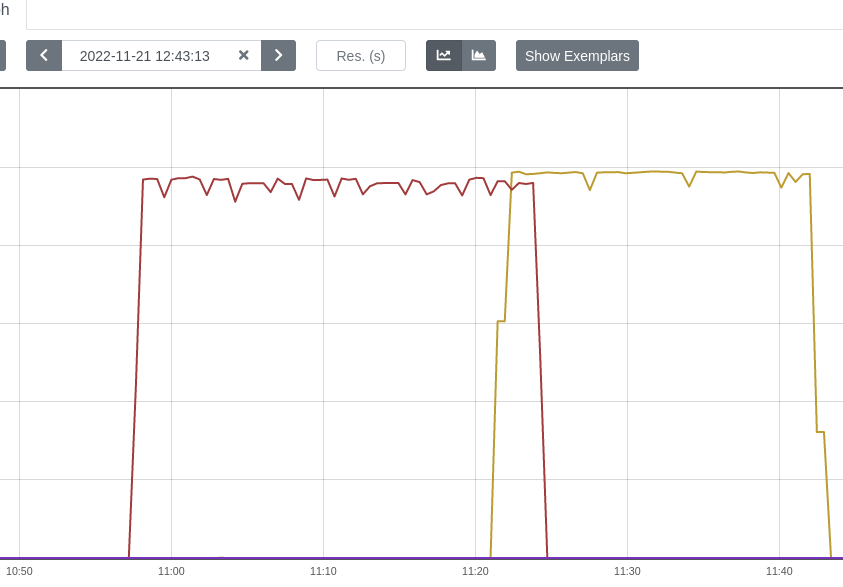
Some other ideas on how to improve GPU utilization:
- Use a smarter dataloader. For example
FFCVloader, but there are many other alternatives. - Use a good profiler to understand what model operations are the most expensive, what is the active CPU time/active GPU time etc. A good starting point is
torch.profiler. Also, one can decide to visualize the profiled operators and CUDA kernels in Chrome trace viewer, to detect performance bottlenecks of the model:
from torch.profiler import profile, ProfilerActivity

with profile(activities=[ProfilerActivity.CPU, ProfilerActivity.CUDA]) as prof:
    trainer.train()

print(prof.key_averages().table(sort_by="cpu_time_total", row_limit=10))
prof.export_chrome_trace("trace.json")
This snippet will export the profiled data into trace.json. Open the generated file with chrome://tracing/ to go into more details about the running processes:
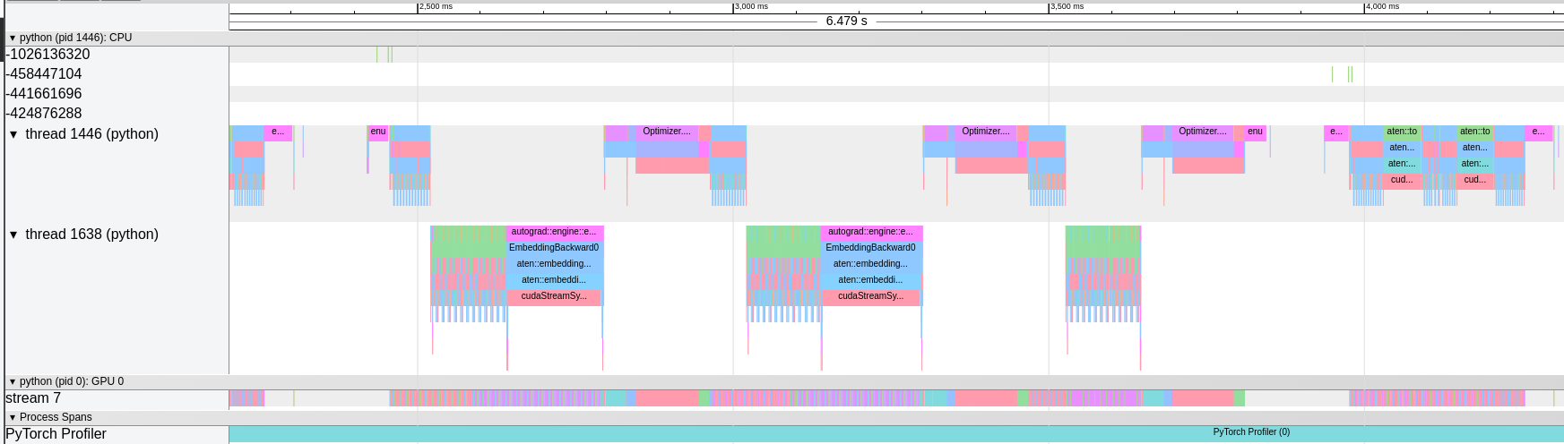
Chrome trace viewer
Environment Setup
The benchmarking is performed exclusively on NVIDIA A100 40GB PCIe GPUs.
For maximum reproducibility, see the exact versions of software used for benchmarking:
- Kubernetes: 1.22
- Container runtime: containerd://1.4.13
- Kubectl: 1.25
- Cuda version utilized: 11.6
- Prometheus: prometheus:v2.28.1
- DCGM image tag: dcgm-exporter:2.4.5-2.6.7-ubuntu20.04
- Node OS image: Fedora CoreOS 35.20220227.2.1
- Node Kernel Version: 5.16.13-200.fc35.x86_64
- Driver Version: 470.129.06
Good to know
NVIDIA System Management Interface (nvidia-smi) is a very handy command line utility to check GPU stats. One nice feature is that it shows what processes are using the GPUs. But this will not work in a containerized setup. nvidia-smi is not compatible with PID namespaces, and as a result will not be able to list the running processes. Compare the outputs:
Output when the GPU is not used, explicitly saying there no running processes.
Output when there is at least a process in a container using the GPU. The section is left empty.
Next episode
In the next blog post, we will dive into the extensive time-slicing benchmarking. Stay tuned!
Efficient Access to Shared GPU Resources: Part 2
This is part 2 of a series of blogposts about GPU concurrency mechanisms. In part 1 we focused on pros and cons and use cases for the different technology solutions available on Kubernetes.
This series focuses on NVIDIA cards, although similar mechanisms might be offered by other vendors.
Introduction
To extend cluster available resources, Kubernetes provides the device plugin framework. It allows specialized hardware to advertise itself to kubelet, without changing or customizing Kubernetes in any way. A high-level overview can be seen below:
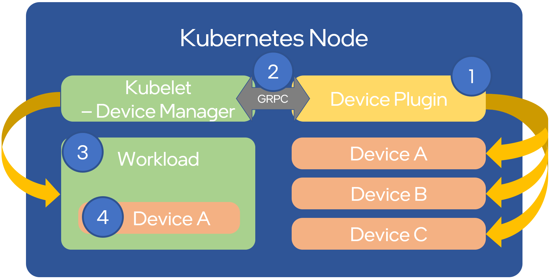
Source: OPNFV
However, configuring the nodes manually and managing them is hard. The administrator will have to deal with drivers, container runtimes, and a wide range of libraries. To simplify this task, NVIDIA provides a way to automate the management of NVIDIA resources and related software using the NVIDIA gpu-operator. This includes NVIDIA drivers, NVIDIA container runtime, Data Center GPU Manager (DCGM) for monitoring, etc. You can read more about this on NGC and GitHub.
Drivers Setup and Configuration
The gpu-operator provides a helm chart allowing basic installation and advanced setup of time-slicing and MIG. We will be doing this with hands-on practice, following each step along the way.
The operator tries to pull an existing container following format <driver>-<name>-<version_id> to install the driver - this must exist in the remote registry. You can check if a tag exists for the specific driver version and distribution you use with:
$ skopeo list-tags -- docker://nvcr.io/nvidia/driver | grep 510.47.03
        "510.47.03-centos7",
        "510.47.03-rhcos4.10",
        "510.47.03-rhcos4.9",
        "510.47.03-ubuntu18.04",
        "510.47.03-ubuntu20.04",
In our case we rely on FCOS which does not have an official image, but there is a fork available in this alternate repository. You can see other available NVIDIA driver version options by filtering the labels by the kernel version.
Armed with our dependent container images, lets install the gpu-operator chart on our cluster. First, add and update the helm chart repo:
$ helm repo add nvidia https://nvidia.github.io/gpu-operator
$ helm repo update nvidia
The gpu-operator appends to the driver image tag -fedora<VERSION_ID>, so we need to mirror the image into our registry. Do this:
$ skopeo copy docker://docker.io/fifofonix/driver:510.47.03-fedora35-5.16.13-200.fc35.x86_64 \
    docker://yourregistry/yourproject/driver:510.47.03-fedora35-5.16.13-200.fc35.x86_64-fedora35 --dest-username <user> --dest-password <password>
Let’s update the gpu-operator values.yaml configuration to meet our expected configuration options:
$ cat values.yaml
operator:
  defaultRuntime: containerd
mig:
  strategy: mixed
driver:
  repository: yourregistry/yourproject
  image: driver
  version: "510.47.03-fedora35-5.16.13-200.fc35.x86_64"
  imagePullPolicy: Always
migManager:
  config:
    name: nvidia-mig-config
devicePlugin:
  config:
    name: nvidia-time-slicing-config
Install with:
$ helm upgrade -i gpu-operator nvidia/gpu-operator --version v22.9.1 --values values.yaml --namespace kube-system
Both driver version and CUDA version can be set using the same values.yaml file provided above. If not explicitly set, the chart will use its own defaults. If setting the versions manually, make sure to check the CUDA Application Compatibility Support Matrix table to choose compatible driver/cuda versions.
To complete the installation, additional files that we will be using will also need to be added. We will explain in the next chapters what these are, but for now download the nvidia-time-slicing-config and nvidia-mig-config manifests and add them to your cluster:
$ kubectl apply -f nvidia-time-slicing-config.yaml
$ kubectl apply -f nvidia-mig-config.yaml
The gpu-operator components should now be installed:
$ kubectl get po -n kube-system
NAME                                                         READY   STATUS      RESTARTS        AGE
nvidia-container-toolkit-daemonset-cb7sj                     1/1     Running     0               3d16h
nvidia-cuda-validator-hkpw7                                  0/1     Completed   0               3d16h
nvidia-dcgm-exporter-vxtx8                                   1/1     Running     0               3d16h
nvidia-device-plugin-daemonset-7cqvs                         2/2     Running     0               2d18h
nvidia-device-plugin-validator-ndk54                         0/1     Completed   0               3d16h
nvidia-driver-daemonset-plzrb                                1/1     Running     0               3d16h
nvidia-hack-force-mig-config-46wrf                           1/1     Running     0               3d16h [1]
nvidia-mig-manager-4szxx                                     1/1     Running     0               3d16h
nvidia-operator-validator-d66nb                              1/1     Running     0               3d16h
[1] On some scenarios, it might be that k8s-device-plugin installation is failing. A workaround manifest is provided.
Time slicing setup on Kubernetes
In the previous post we introduced time slicing and its particularities. The gpu-operator brings a default configuration for the slicing profiles. Below we give an example to add custom profiles allowing GPUs to be shared between 4 or 10 pods. This is done by specifying that the resource of type nvidia.com/gpu is split into 4 or 10 replicas and can be shared among 4 or 10 pods:
apiVersion: v1
kind: ConfigMap
metadata:
  name: nvidia-time-slicing-config
  namespace: kube-system
data:
  slice-4: |-
    version: v1
    sharing:
      timeSlicing:
        renameByDefault: true
        failRequestsGreaterThanOne: true
        resources:
        - name: nvidia.com/gpu
          replicas: 4
  slice-10: |-
    version: v1
    sharing:
      timeSlicing:
        renameByDefault: true
        failRequestsGreaterThanOne: true
        resources:
        - name: nvidia.com/gpu
          replicas: 10
The configuration in the previous section already included the reference to this configmap.
Once you’ve updated the configuration, you can:
- Apply it to existing nodes with an explicit label:
$ kubectl label node <NAME> nvidia.com/device-plugin.config=<PROFILE>
- Set a default profile for every GPU node on your cluster, by passing it in the helm chart config:
devicePlugin:
  config:
    default: <PROFILE>
Let’s set now a time-slice profile on one of our nodes. Reconciliation should take 1 to 2 minutes:
$ kubectl label node <NAME> nvidia.com/device-plugin.config=slice-4
To verify the time sharing is enabled after labeling, use the kubectl describe node command. Check the GPU number in the allocatable resources section, it should have changed to 4 times the nodes physical available GPUs. With our time-slicing configuration the new resource will be appended .shared. So, on a node with 4 GPU cards:
Allocatable:
  nvidia.com/gpu: 4
Becomes:
Allocatable:
  nvidia.com/gpu.shared: 16
Test that the deployment is working as expected with a test manifest:
apiVersion: apps/v1
kind: ReplicaSet
metadata:
  name: nvidia-test-time-slice
  labels:
    app: nvidia-test
spec:
  replicas: 5
  selector:
    matchLabels:
      app: nvidia-test
  template:
    metadata:
      labels:
        app: nvidia-test
    spec:
      containers:
      - name: nvidia
        image: oguzpastirmaci/gpu-burn
        args:
        - "10000"
        resources:
          limits:
              nvidia.com/gpu.shared: 1
$ kubectl get po
NAMESPACE       NAME                                                         READY   STATUS      RESTARTS       AGE
default         nvidia-test-time-slice-2jxt2                                 1/1     Running     0              22s
default         nvidia-test-time-slice-gzxr5                                 1/1     Running     0              22s
default         nvidia-test-time-slice-kpwcn                                 1/1     Running     0              22s
default         nvidia-test-time-slice-vt265                                 1/1     Running     0              22s
default         nvidia-test-time-slice-wvpx4                                 1/1     Running     0              22s
…
The time slicing capabilities can be used together with MIG. Simply pass a MIG instance (for example nvidia.com/mig-1g.5gb) instead of the generic nvidia.com/gpu. The next section will cover the MIG setup.
Check the official Nvidia docs for most information on GPU time slicing.
Limiting Memory Usage
As described in part1, one of the major limitations of Time Slicing is the lack of memory isolation between GPU processes that run on the same card. This can be limited on some frameworks like Tensorflow but it depends on the users respecting declared resources.
To mitigate bad actors from interfering with other users GPU processes by starving the card out of memory (past the agreed maximum memory) we use a simple process that periodically watches and monitors the GPU process allocated memory and kills any outliers. This is similar to what Kubernetes does to control memory usage by pods.
Ensuring any running process on the GPU respects the agreed memory allows us to provide a more reliable environment for development workloads like notebooks or other typically spiky workloads, while improving overall usage and efficiency of individual cards.
Multi Instance GPU Setup on Kubernetes
In the previous post we introduced MIG, some of its particularities and use cases. In addition, when using MIG, there are multiple strategies available:
- single:
- MIG devices are enumerated as nvidia.com/gpu.
- The resource nvidia.com/gpu now maps to the MIG devices available on that node, instead of the full GPUs.
- mixed:
- Different resource types are enumerated for every MIG device available. Ex: nvidia.com/mig-3g.20gb, nvidia.com/mig-1g.5gb, etc.
- The partitions can be requested by name.
- mig.strategy should be set to mixed when MIG mode is not enabled on all GPUs on a node.
- none:
- No distinction between GPUs with MIG or without. The available devices are listed as nvidia.com/gpu resource type.
Similarly to the time-slicing configuration file, the gpu-operator brings a default configuration for the MIG profiles, but we will create one ourselves to allow some customizations - in this example we ignore things we do not consider useful (for example 7g.5gb). A snippet of our full configmap is described below:
apiVersion: v1
kind: ConfigMap
metadata:
  name: nvidia-mig-config
  namespace: kube-system
data:
  config.yaml: |
    version: v1
    mig-configs:
      disabled:
      - devices: all
        mig-enabled: false

      # A100-40GB
      2x2g.10gb-3x1g.5gb:
      - devices: all
        mig-enabled: true
        mig-devices:
          "1g.5gb": 3
          "2g.10gb": 2
A complete list of A100 GPUs MIG profiles can be found in the documentation, but not all configurations are exposed by us. Only the ones that optimize compute performance. This will be addressed in a future blogpost.
In the Drivers Setup and Configuration section, in values.yaml for the gpu-operator, the mig strategy was already set to mixed. So, the next step is to choose the profile for each node via a label:
$ kubectl label node <NAME> nvidia.com/mig.config=<PROFILE>
For example, if a node has 4 A100 GPUs available, and is labeled with nvidia.com/mig.config=7x1g.5gb all GPUs in that node will be partitioned into 7 MIG graphical instances. Depending on the type of strategy selected on the node, the allocatable.resources publicized by that node will be:
- for single strategy: 4*7 = 28
nvidia.com/gpu - for mixed strategy: 4*7 = 28
nvidia.com/mig-1g.5gb
More information can be found in the GPU operator and MIG user guide upstream documentation.
Here’s an example setting the 2x2g.10gb-3x1g.5gb MIG profile to one node:
$ kubectl label node <NAME> nvidia.com/mig.config=2x2g.10gb-3x1g.5gb
So, on a node with 4 GPU cards:
Allocatable:
  nvidia.com/gpu: 4
Becomes:
Allocatable:
  nvidia.com/mig-1g.5gb: 12
  nvidia.com/mig-2g.10gb: 8
Test that the deployment is working as expected with a test manifest:
apiVersion: apps/v1
kind: ReplicaSet
metadata:
  name: nvidia-test-mig-a100
  labels:
    app: nvidia-test
spec:
  replicas: 4
  selector:
    matchLabels:
      app: nvidia-test
  template:
    metadata:
      labels:
        app: nvidia-test
    spec:
      containers:
      - name: nvidia
        image: oguzpastirmaci/gpu-burn
        args:
        - "10000"
        resources:
          limits:
              nvidia.com/mig-2g.10gb: 1
$ kubectl get po
NAME                          READY   STATUS    RESTARTS   AGE
nvidia-test-mig-a100-bw95c    1/1     Running   0          78s
nvidia-test-mig-a100-drxg5    1/1     Running   0          78s
nvidia-test-mig-a100-kk5wb    1/1     Running   0          78s
nvidia-test-mig-a100-n9mbr    1/1     Running   0          78s
Monitoring your cluster
With a variety of GPU Cards and different working mechanisms that can be used, it is important to keep track of the resource usage to know if the resources are not idling when otherwise they can be re-assigned.
Using the gpu-operator and enabling monitoring with prometheus by using the kube-prometheus-stack helm chart you can collect the metrics made available by the NVIDIA DCGM exporter. Internally we created a dashboard to showcase resource usage on clusters supporting heterogeneous nodes and different mechanisms. You can find it in the upstream grafana dashboards repository.

Source: CERN
While CUDA cores are designed for general-purpose parallel computing, Tensor cores are specialized for deep learning and AI. As a result, not all workloads will benefit from them. In this context, to make sure the GPU is fully utilized, it is a good idea to have more granular cores utilization monitoring, as presented in the image below:
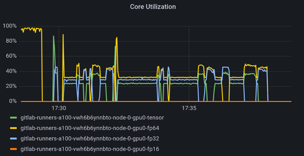
Source: CERN
Conclusions
As you could see, installing and configuring your Kubernetes cluster to be able to use NVIDIA GPU’s is quite simple due to the usage of the NVIDIA provided gpu-operator helm chart. Some details need to be taken into account due to the underlying host kernel and OS being used so that the compatible kernel modules can be used/compiled.
In this section we have shown how to use time-slicing and MIG configuration on the cluster nodes. For more advanced deployments the cluster administrator can also configure time-slicing on top of MIG GPU instances, but this was not demonstrated here.
Because we are labeling each node individually we can have coexistence of different configurations - full card, time-slice and MIG - in a single cluster. This is useful if we have a cluster with heterogeneous card types (T4, A100, …) and we want to accommodate different profiles to optimize cluster resource usage.
Next Episode
With the configurations provided in this blog post we’re ready to test our deployments. In the next blog post we will provide performance benchmarks using different configurations and profiles. Stay tuned!
Efficient Access to Shared GPU Resources: Part 1
GPUs are shaping the way organizations access and use their data and CERN is not an exception. Traditional High Energy Physics (HEP) analysis and deployments are being rethought and accelerators remain the key to enabling efficient Machine Learning (ML).
In this series of blog posts we will cover the use cases and technologies that motivate and enable efficient sharing of GPUs on Kubernetes. For both on-premises and public cloud (on demand) access to accelerators, this can be a key factor for a cost effective use of these resources.
This post focuses on NVIDIA cards, similar mechanisms might be offered by other vendors.
Motivation
CERN’s main facility today is the Large Hadron Collider. Its experiments generate billions of particle collisions per second, with these numbers about to grow with planned upgrades. The result are hundreds of PetaBytes of data to be reconstructed and analized using large amounts of computing resources.


Even more data is generated from physics simulation which remains a cost effective way to guide the design and optimization of these giant machines as well as a basis to compare results with a well defined physics model.
GPUs are taking a central role in different areas:
- As a more efficient replacement for traditional CPU cores in simulation, or even to replace custom hardware with more flexible resources in online triggers.
- In ML for particle classification during event reconstruction (GNN), much faster generation of simulation data (3DGAN), reinforcement learning for beam calibration, among others.
As demand grows one important aspect is to ensure this type of (expensive) hardware is optimally utilized. This can be a challenge given:
- Workloads are often not capable of taking full advantage of the resources due to usage patterns, suboptimal code, etc. As with CPU virtualization, enabling resource sharing can mitigate this loss.
- Many of these workloads are spiky which can trigger significant waste if resources are locked for long periods. This is often the case during the interactive and development phase of the different components, or for services with uneven load.
Kubernetes has had support for different types of GPUs for a while now although not as first class resources and limited to dedicated, full card allocation. With the demand growing and Kubernetes established as the de-facto platform in many areas, multiple solutions exist today to enable concurrent access to GPU resources from independent workloads.
It is essential to understand each solution’s benefits and tradeoffs to enable an informed decision.
GPU Concurrency Mechanisms
By concurrency we mean going beyond simple GPU sharing. GPU sharing includes deployments where a given pool of GPUs is shared but each card is assigned to only one workload at a time for a limited (or not) amount of time.
The figure below summarizes the multiple concurrency options with NVIDIA cards.
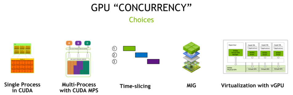
Source: NVIDIA
Out of the different mechanisms above we will not cover those that are CUDA-specific (single and multiple process CUDA) and will briefly cover the possibility of simply co-locating workloads on a single card.
Co-located Workloads
Co-locating workloads refers to uncontrolled access to a single GPU. At CERN an example of such offering is the lxplus interactive service which has dedicated nodes with GPUs. Users login to shared virtual machines each exposing a single card via PCI passthrough.
Advantages:
- The easiest way to provide GPU concurrency.
- Works by simply exposing the card via PCI passthrough.
Disadvantages:
- No memory isolation, regular OOM errors for workloads.
- Unpredictable performance.
- Limited control over the number of workloads using the GPU.
- Monitoring only of the full card, not workload specific.
Time Slicing
Time Slicing is a mechanism that allows multiple processes to be scheduled on the same GPU. The scheduler will give an equal share of time to all GPU processes and alternate in a round-robin fashion.
As a result, if the number of processes competing for resources increases, the waiting time for a single process to be re-scheduled increases as well. Below is a simplified timeline for 4 processes running on a shared GPU.
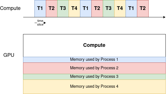
The memory is divided between the processes, while the compute resources are assigned to one process at a time.
Advantages:
- A very easy way to set up GPU concurrency.
- An unlimited number of partitions.
- Works on a very wide range of NVIDIA architectures.
Disadvantages:
- Unused computational resources remain idle during each time slice.
- No process or memory isolation, a single user can claim all memory and OOM others.
- Inappropriate for latency-sensitive applications, like for example desktop rendering for CAD workloads.
- No ability to set priorities or size slices of resources available for each workload. The time-slice period is a constant value across processes.
- Performance drop to be expected (more later in this series of blog posts).
Virtual GPU (vGPU)
vGPUs is an enterprise software from NVIDIA allowing GPU concurrency. It can be installed on GPUs in data centers or cloud and is often used to allow multiple virtual machines to access a single physical GPU.
NVIDIA provides 4 vGPU options based on different needs.
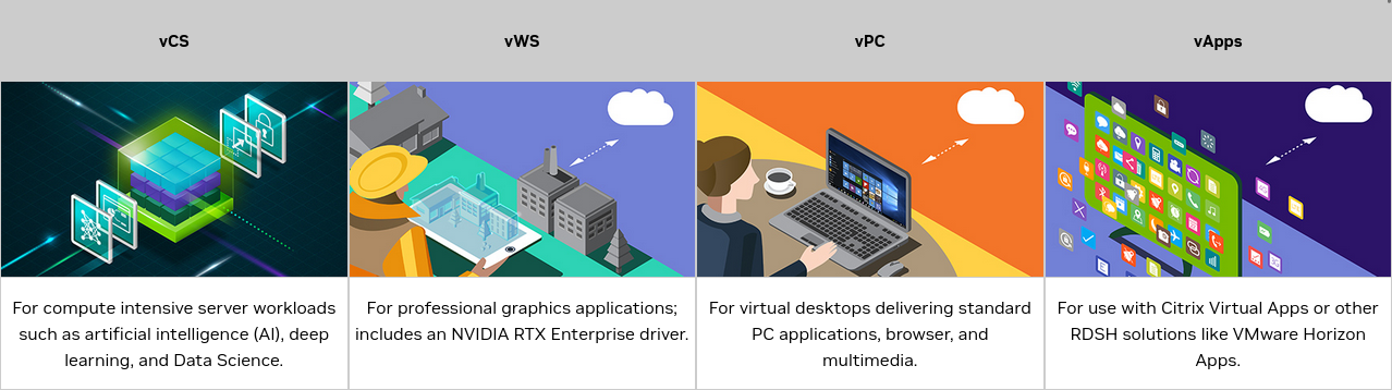
Source: NVIDIA
Advantages:
- Offers both memory bandwidth QoS and monitoring and telemetry capabilities for individual virtual partitions.
- Allows different scheduling policies, including best-effort, equal share and fixed share.
- Availability for earlier NVIDIA generations (Maxwell, Pascal and Volta in addition to more recent ones).
- Predictable performance when using fixed share scheduler.
Disadvantages:
- Enterprise solution, requires an additional license from NVIDIA.
- Performance loss due to virtualization.
- Requires a specific driver running on hypervisors.
- Partitioning still done via time-slicing, with processes being run serially and preempted at every time slice.
- No hardware isolation between workloads.
Multi-Instance GPU (MIG)
MIG technology allows hardware partitioning a GPU into up to 7 instances. Each instance has isolated memory, cache, bandwidth, and compute cores, alleviating the “noisy neighbour” problem when sharing a GPU. At the time of writing, it is available for Ampere and Hopper architecture.
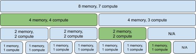
Source: Patterson Consulting
The smallest partition of the GPU is called a slice and consists of 1/8 of the memory and 1/7 of Streaming Multiprocessors (SMs) - the component that executes compute instructions on the GPU.
The possible combinations of slices are shown in the figure above, and are often referred to as Xg.Ygb denoting X compute slices and Y total memory. It is possible to mix different profiles in the same card, as denoted in green above.
Advantages:
- Hardware isolation, mean concurrent processes run securely and do not influence each other.
- Monitoring and telemetry data available at partition level.
- Allows partitioning based on use cases, making the solution very flexible.
Disadvantages:
- Only available for Ampere and Hopper architecture (as of early 2023).
- Reconfiguring the partition layout requires all running processes being evicted.
- Loss of SM cores when enabling MIG (more details to follow in our series).
- Potential loss of available memory depending on profile layout chosen.
How To Choose
Making a choice in favor of a concurrency mechanism can be hard. Depending on your use case and the resources at your disposal, the table below will help you choose the most appropriate configuration for your use case:
A big part of the table is taken from this source. Consult it for more information.
Features
| Time slicing | vGPU | MIG | |
|---|---|---|---|
| Max Partitions | Unlimited | Variable (flavor and card) | 7 |
| Partition Type | Temporal | Temporal & Physical (VMs) | Physical |
| Memory Bandwidth QoS | No | Yes | Yes |
| Telemetry | No | Yes | Yes |
| Hardware Isolation | No | No | Yes |
| Predictable Performance | No | Possible¹ | Yes |
| Reconfiguration | Not applicable | Not Applicable | When idle |
Use Cases
| Examples | Time slicing | vGPU | MIG | |
|---|---|---|---|---|
| Latency-sensitive | CAD, Engineering Applications | No | Possible¹ | Yes |
| Interactive | Notebooks | Yes² | Yes | Yes |
| Performance intensive | Simulation | No | No | Yes |
| Low priority | CI Runners | Yes | Yes (but not cost-effective) | Yes |
¹ When using the fixed share scheduler.
² Independent workloads can trigger OOM errors between each other. Needs an external mechanism to control memory usage (similar to kubelet CPU memory checks).
Support on Kubernetes
Kubernetes support for NVIDIA GPUs is provided with the NVIDIA GPU Operator.
How to use it and configure each of the concurrency mechanisms discussed will be the topic of the next post in this series.
Announcing CVMFS CSI v2
We are glad to announce the release of cvmfs-csi v2.0.0 bringing several cool features and making access to CVMFS repositories inside Kubernetes a lot easier. This is a large overhaul of the first version of the driver, see below for some history and details of how things improved.
What is CVMFS
CVMFS is the CernVM File System. A scalable, reliable and low-maintenance software distribution service developed to assist high energy physics experiments to deploy software on the worldwide distributed computing grid infrastructure.
It exposes a POSIX read-only filesystem in user space via a FUSE module, with a universal namespace - /cvmfs - and the backend relying on a hierarchical structure of standard web servers.
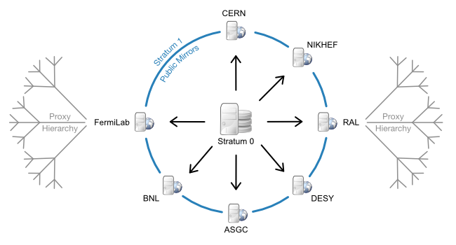
Exposing CVMFS repositories to containerized deployments, first with Docker and then Kubernetes, has been one of our first requirements.
First integration: Docker and FlexVolume
The first integration in the early container days at CERN included a docker volume plugin and right after the integration with Kubernetes via a FlexVolume. A Kubernetes manifest was similar to any other volume type:
volumes:
- name: atlas
  flexVolume:
    driver: "cern/cvmfs"
    options:
      repository: "atlas.cern.ch"
After defining a flexVolume volume in a Pod spec users could access the CVMFS repository from within their application. This worked well and for Kubernetes 1.6 this was the best way of exposing storage systems that didn’t have direct, in-tree support inside Kubernetes. However, the design of the FlexVolume plugin API itself had many limitations. For example:
- The API offered only attaching and mounting
- The plugin(s) had to be available on nodes where they’d be run directly by kubelet
- It was assumed that all mount dependencies (mount and filesystem tools) these plugins used were available on the host
For these reasons and others the Flex volume plugins were later deprecated, making the CVMFS FlexVolume plugin no longer a viable option.
Second Round: Arrival of CSI
Things changed with the arrival of the CSI (Container Storage Interface) in 2017, developed as a standard for exposing arbitrary block and file storage systems to containerized workloads on systems like Kubernetes.
Once the interface got a bit more stable we created a CSI driver for CVMFS, with the first release in 2018 offering mounts of single CVMFS repositories. This involved defining both a StorageClass and a PersistentVolumeClaim as in this example:
apiVersion: storage.k8s.io/v1
kind: StorageClass
metadata:
  name: csi-cvmfs-cms
provisioner: cvmfs.csi.cern.ch
parameters:
  # Repository address.
  repository: cms.cern.ch
---
apiVersion: v1
kind: PersistentVolumeClaim
metadata:
  name: csi-cvmfs-cms-pvc
spec:
  accessModes:
  - ReadOnlyMany
  resources:
    requests:
      # The volume size is arbitrary as it is ignored by the driver.
      storage: 1Gi
  storageClassName: csi-cvmfs-cms
Pods would then mount it like any other PVC. For simple setups this was good enough but for applications that use many repositories this quickly becomes hard to scale, as:
- The number of PVCs is proportional to the number of CVMFS repositories used
- The list of repositories must be known during deployment time of application Pods
- The client configuration is loaded only during deployment time of the driver
Previous alternatives
Due to the missing features and faults of the first version of the CSI driver a few alternatives appeared in the community: CERN Sciencebox CVMFS driver, PRP OSG driver, docker-cvmfs to name a few.
All of these are designed similarly with a DaemonSet deployment exposing /cvmfs or individual repositories on a hostPath, and application mounting them from the host. This approach works well enough for many cases, but misses things like declaring them explicitly as PersistentVolumes, full integration and validation with the Kubernetes storage stack, reporting of failed mounts, monitoring, etc.
Many deployments also prevent usage of hostPath from user Pods.
Meet cvmfs-csi v2
The new CSI driver tackles all the issues above, with the main feature being the introduction of automounts. With one PVC users can now mount any and all repositories, on-demand, just by accessing them.
Here’s an example manifest:
apiVersion: storage.k8s.io/v1
kind: StorageClass
metadata:
  name: cvmfs
provisioner: cvmfs.csi.cern.ch
---
apiVersion: v1
kind: PersistentVolumeClaim
metadata:
  name: cvmfs
spec:
  accessModes:
  - ReadOnlyMany
  resources:
    requests:
      # Volume size value has no effect and is ignored
      # by the driver, but must be non-zero.
      storage: 1
  storageClassName: cvmfs
---
apiVersion: v1
kind: Pod
metadata:
  name: cvmfs-demo
spec:
  containers:
   - name: nginx
     image: nginx
     imagePullPolicy: IfNotPresent
     volumeMounts:
       - name: my-cvmfs
         mountPath: /my-cvmfs
         # CVMFS automount volumes must be mounted with HostToContainer mount propagation.
         mountPropagation: HostToContainer
  volumes:
   - name: my-cvmfs
     persistentVolumeClaim:
       claimName: cvmfs
The StorageClass cvmfs is pre-defined in CERN Kubernetes clusters.
After creating the cvmfs-demo Pod, repositories can be accessed like so:
$ kubectl exec -it cvmfs-demo -- /bin/sh
~ # ls -l /my-cvmfs
total 0
Note no content is shown in the directory as no repo has been accessed yet. They are loaded on demand the first time they are requested, like shown in these examples for atlas.cern.ch and cms.cern.ch:
~ # ls -l /my-cvmfs/atlas.cern.ch
total 1
drwxr-xr-x   10 999      997             16 Feb 29  2020 repo

~ # ls -l /my-cvmfs/cms.cern.ch
total 1282
drwxr-xr-x    8 999      997              4 Aug 19  2015 CMS@Home
drwxr-xr-x   19 999      997           4096 Apr 11 08:02 COMP
-rw-rw-r--    1 999      997            429 Feb 12  2016 README
-rw-rw-r--    1 999      997            282 Feb 18  2014 README.cmssw.git
-rw-rw-r--    1 999      997             61 Jul 13  2016 README.grid
-rw-r--r--    1 999      997            341 Apr 23  2019 README.lhapdf
...
Another big change in the new version is the support for multiple CVMFS client configurations via a ConfigMap. Previously this could only be done in the driver deployment configuration, meaning a restart of the CSI driver was needed. With the new version once the ConfigMap is updated all new mounts can rely on the new settings, with no impact on existing mounts. Here’s an example for the DESY instance:
data:
  ilc.desy.de.conf: |
    CVMFS_SERVER_URL='http://grid-cvmfs-one.desy.de:8000/cvmfs/@fqrn@;...'
    CVMFS_PUBLIC_KEY='/etc/cvmfs/config.d/ilc.desy.de.pub'
  ilc.desy.de.pub: |
    -----BEGIN PUBLIC KEY-----
    MIIBIjANBgkqhkiG9w0BAQEFAAOCAQ8AMIIBCgKCAQEA3pgrEIimdCPWG9cuhQ0d
    ...
    -----END PUBLIC KEY-----
Next steps
We still want to continue evolving the plugin. The immediate focus will be on:
- Support for Volume Health Monitoring to detect abnormal volume conditions and report them as events to the
PVCsorPods - (Re)Add support for CVMFS
TagsandHashes, a feature that was present in the previous driver version but that is not very popular among CVMFS users – according to the CVMFS team this is barely used, if at all. Still, we would like to make sure we support this in the near future
If you are a user of the CERN Kubernetes service, the new driver is available in all cluster templates for Kubernetes >=1.24. Check out our docs.
If you have other Kubernetes deployments and need access to CVMFS repos, please try the new version and give any feedback in our new home! The driver now lives next to the CVMFS core components, where it belongs.
A Summer of Testing and Chaos
After two years of an imposed remote only version, CERN welcomed again a large number of newcomers for the summer student and openlab summer programs. This time two of them will be working in our Kubernetes service team.

They’ll be jumping in and out of physics and computing lectures, working on their projects and hopefully having a lot of fun!
Welcome Vitor
Vitor comes from Sao Paulo in Brazil where he studies computing engineering. He will focus on improving our service’s functional testing infrastructure using some well known tools in the cloud native space.
From our current limited visualization,
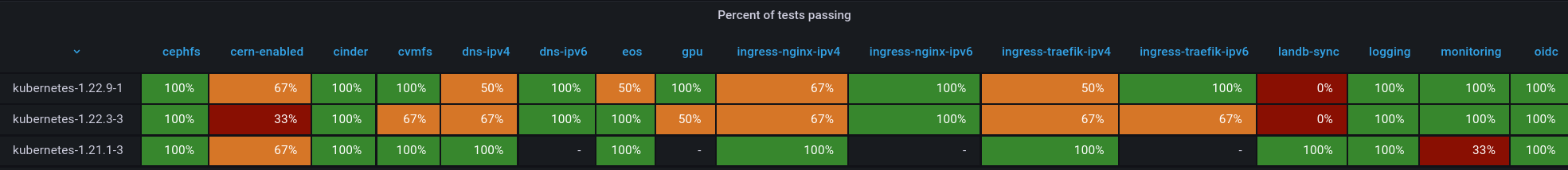
Vitor will be checking how a move to Argo Workflows could help us with a number of items we’ve wanted to improved for quite some time:
- Better way to declare the test scenarios and their relationships and dependencies on other services in CERN IT
- Faster access to test run logs from services and infrastructure nodes
- Easy reproducibility of test failures, particularly manual runs of failed steps
Welcome Nivedita
Nivedita comes from Siliguri in India and is already very involved in the upstream Kubernetes community - she’s part of the Kubernetes 1.25 release team (yay!) after having done it for 1.24 as well.
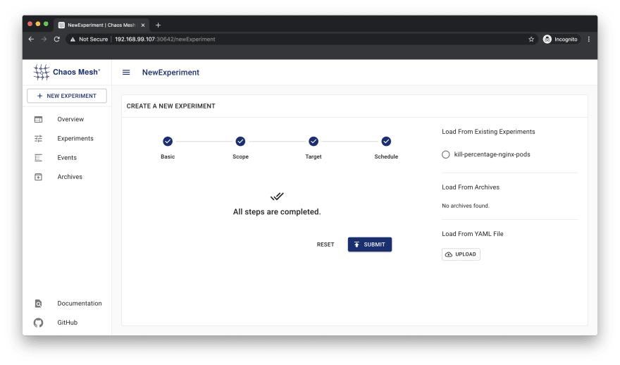
Her focus will be on an add-on to our cluster deployments enabling Chaos Engineering, made popular long ago by the Netflix Chaos Monkey. This will be the next step in our years-long quest for improved service availability, making us more comfortable with enabling regular experiments triggering failures across the fleet. So the days things break for real, we won’t notice.
Check this space again in September for some exciting progress. It’s summer time!
Summary of the GitOps Workshop
On April 27th we had our Kubernetes GitOps Workshop at CERN, with 130 people attending both in-person and virtually. Slides as well as the full recording of the event are available.
Starting from the end here’s a list of the expected follow up actions:
- Agree on a recommendation for managing secrets and other sensitive data. Options presented included SealedSecrets, Mozilla SOPS with different plugins (Barbican, Age, …) and others. In general the audience agreed a central Vault offering would be the key to improve integration with other tools
- Group together the different teams relying on Flux and ArgoCD. The goal is not to recommend one over the other but to document differences and come up with documentation and best practices for each of the solutions
Some details below from the different sessions in the workshop.
Kicking off the day we had Benjamin Bergia from RCS-SIS presenting their integration with GitHub Actions triggering cluster updates with ArgoCD and Kustomize, along with their repository structure and workflows.
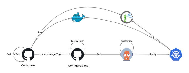
He highlighted the speed of getting things done, and the challenge of choosing the right directory structure for your own needs and some release compatibility issues with upstream Kustomize.
Next we heard from Arthur Outhenin-Chalandre from the CEPH team describing his home setup with k3s and a variety of useful CNCF projects providing networking, logging and monitoring. Plus helm libraries and charts for fun and profit…
Luca Bello from the MONIT team went through their setup with a very well established stack relying on Flux2, Helm3, GitLab CI and SOPS handling sensitive data in git.
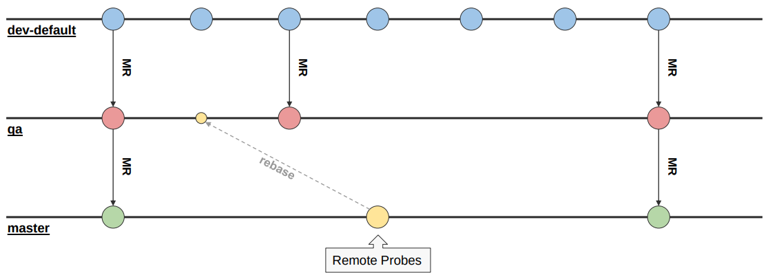
He also provided details on how they split clusters and manage different environments in a single cluster, which add-ons they install everywhere and the workflows and release process. The SOPS usage in particular triggered several questions from the audience.
After a short break we heard from Radu Carpa from the ATLAS Rucio team describing their migration from Puppet to Kubernetes, and some interesting details for cluster bootstrapping using terraform - and how that is one of the current pain points. Radu live demoed their production repositories, and presented a now familiar stack with Flux2, SOPS and Kustomize. Discussion went around terraform usage, private key handling with SOPS and automation of AlertManager configurations.
Jack and Konstantinos from the OpenShift team were up next presenting the usage of GitOps in the OpenShift deployments, and more specifically for the Drupal deployments at CERN.
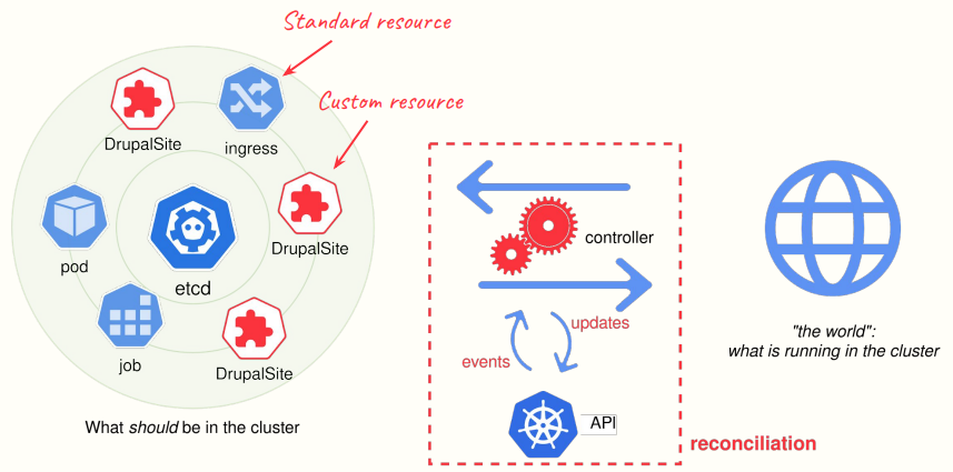
They explained how they achieve continuous delivery with a custom resource definition (CRD) and a corresponding operator, all managed via GitOps. They also highlighted the wish for a central Vault deployment to ease the management of sensitive data.
Next up we had Antonio and Ioannis from the JEEDY team describing how GitOps replaced their previous setup with Rundeck managing remote deployments, improving traceability, versioning and the ability to rollback changes. They demoed how changes in a Git repo are quickly propagated to the different clusters, and as for next steps from their point of view these would include: improved secret management, cluster management also using ArgoCD, notifications and extending usage to other applications.
The final session of the day covered the multiple options to manage secrets, and it worked as a good kickstart for the follow up discussion. Highlights include (but do check the recording):
- What’s the best way to handle secrets and other sensitive data? Lots of different options were presented, with SOPS being the most popular. But even then SOPS is the library for managing secrets, not the secret store itself. Focusing on getting a central Vault offering available from CERN IT, and some best practices on how to integrate it with Kubernetes should be a priority
- Is Terraform enough of a pain point to invest in something like Crossplane? Some work expected in the next couple months to add an OpenStack provider to Crossplane
- Should people use Flux or ArgoCD? The presentations showed that users of both tools are happy with their choice, and hinted that the way forward might be to strengthen the user communities behind them to ensure proper documentation and best practices. Future will tell if one ends up taking over the majority of deployments
- What is the best communication channel to discuss these and similar issues? The consensus was that the Cloud Containers channel on mattermost is currently the best place
And that was it. A morning packed with content and several actions to be followed up.
See you next time!
GitOps Workshop
GitOps is a set of practices to manage infrastructure and application configurations using Git. It relies on Git as a single source of truth for declarative infrastructure and applications, and a set of reconcilers to apply changes.
Workshop goals:
- Assess the usage of GitOps in the Kubernetes/OpenShift community at CERN
- Share experiences on usage of the multiple GitOps tools, including ArgoCD, Flux (v1 and v2), GitLab CI or even custom deployment scripts around tools like Helm
- Consider consolidation of these efforts moving forward
If you are a user of such systems, please consider submitting an abstract with a title and a small description the tools and workflows you rely on to automate your deployments.
In addition to presentations there will be plenty of time for general discussion.
Kubernetes Deprecations and Removals v1.20/21/22
The latest Kubernetes version (v1.20) and the next two releases will bring deprecations and removals of resources and APIs still in use by multiple applications. This is also related to the upstream community decision to avoid APIs remaining permanently in beta.
Please review your deployments to ensure you can smoothly move your applications to new cluster versions in the future. The list below includes the most relevant changes coming up in the near future:
v1.20
- PodPreset is dropped completely. Alternatives include Mutating Admission Webhooks
v1.21
- PodSecurityPolicy deprecation (to be removed completely in 1.25). Alternatives include the Open Policy Agent (OPA) and Validating Admission WebHooks
v1.22
- Removal of extensions/v1beta1 Ingress, moved to networking.k8s.io/v1 (stable API)